Table of Contents

• Coursera Course overview
• Other resources
• Sequence models
• Recurrent Neural Networks
  • Unidirectional RNN
  • Forward propagation
  • Backpropagation
  • RNN architectures
    • Encoder-Decoder Networks
  • Language model and sequence generation
  • Vanishing Gradients in RNN
    • Gated Recurrent Units
      • Simple GRU
      • Full GRU
    • Long Short Term Memory Units
    • GRU vs. LSTM
  • Bidirectional RNNs
  • Deep RNN
• Natural Language Processing
  • Properties of word embeddings
  • Embedding matrix
  • Word2Vec
    • Skip-Gram
    • Negative Sampling
  • GloVe
  • Sentiment classification
  • Debiasing Word Embeddings
• Sequence-to-sequence models
  • S2S in machine translation
  • Beam search
    • Refinements to Beam Search
      • Length normalization
      • Error Analysis
    • Bleu Score
• Attention models
• Speech recognition
  • Trigger word detection

Coursera Course overview

In the first week you know Recurrent Neural Networks (RNN) as a special form of NN and what types of problems they’re good at. You also learn why a traditional NN is not suitable for these kinds of problems. In the first week’s assignment you will implement two generative models: a RNN that can generate music that sounds like a Jazz improvisation. You also implement another form of an RNN that uses textual input to generate random names for dinosaurs. The second week is all about Natural Language Processing (NLP). You learn how word embeddings can help you with NLP tasks and how you can deal with bias. In the second week you will implement some core functions of NLP models such as calculating the similarity between two words or removing the gender bias. You will also implement a RNN that can classify an arbitrary text with a suitable Emoji. The last and final week of this specialization introduces the concept of Attention Models as a special form of Sequence-to-Sequence models and how they can be used for machine translation. You will put your newly learned knowledge about Attention Models into practice by implementing some functions of an RNN that can be used for machine translation. You will also learn how to implement a model that is able to detect trigger words from audio clips.

Other resources

Description	Link
Adam Coates giving a lecture about speech recognition. Some topics of this page are covered. If you’re not in the mood for reading, watch this! Fun fact: at 0:13 you can see Andrew Ng sneak in	YouTube
What does it really mean for a robot to be racist?: Why bias can become a problem in language models	thegradient.pub
Why bias matters and how to mitigate it.	Google Developers Blog
The Unreasonable Effectiveness of Recurrent Neural Networks: Why RNNs are cool	karpathy.github.io

Sequence models

The previously seen models processed some sort of input (e.g. images) which exhibited following properties:

• it was uniform (e.g. an image of a certain size)
• it was processed as a whole (i.e. an image was not partially processed)
• it was often multidimensional (e.g. an image with 3 color channels yields a matrix of $B \times H \times 3$)

Sequence models are a bit different in that they require their input to be a sequence of tokens. Examples for such sequences could be:

• audio data (sequence of sounds)
• text (sequence of words)
• video (sequence of images)
• …

The length of the individual input elements (i.e. their number of tokens) does not need to be of the same length, neither for training nor prediction. These input tokens are processed one after the other, whereas at each time step a certain token is processed. Processing can be stopped at any point. A form of sequence models are Recurrent Neural Networks (RNN) which are often used to process speech data (e.g. speech recognition, machine translation), generative models (e.g. generating music) or NLP (e.g. sentiment analysis, named entity recognition (NER), …).

The notation for an input sequence $x$ of length $T_x$ or an output sequence $y$ of length $T_y$ is as follows (note the new notation with chevrons around the indices to enumerate the tokens):

$$x = x^{<1>}, x^{<2>}, ..., x^{<t>}, ..., x^{<T_x>} \\ y = y^{<1>}, y^{<2>}, ..., y^{<t>}, ..., y^{<T_y>}$$

As stated above, the input and the output sequence don’t need to be of the same length ($T_x^{(i)} \neq T_y^{(i)}$). Also the length of the individual training samples can vary ($T_y^{(i)} \neq T_y^{(j)}$).

Recurrent Neural Networks

The previously seen approach of a NN with an input layer, several hidden layers and an output layer is not feasible for the following reasons:

• input and output can have different lengths for each sample (e.g. sentences with different numbers of words)
• the samples don’t share common features (e.g. in NER, where the named entity can be at any position in the sentence)

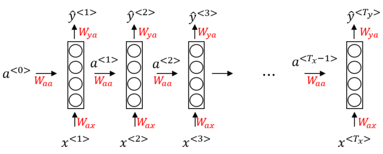
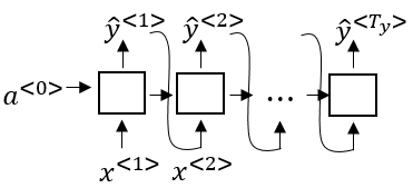
Because RNN process their input token by token they don’t suffer from these disadvantages. A simple RNN only has one layer through which the tokens pass during training/processing. However, the result of this processing has an influence on the processing of the next token. Consider the following sample architecture of a simple RNN:

A side effect of this kind of processing is that an RNN requires far less parameters to be optimized than e.g. a ConvNet would to do the same task. This especially comes in handy for sentence processing where each word (token) can be a vector of dimension e.g. $10'000 \times 1$.

Unidirectional RNN

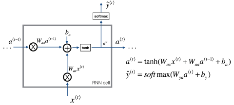
As seen in the picture above the RNN processes each token $x^{<t>}$ individually from left to right, one after the other. In each step $t$ the RNN tries to predict the output $\hat{y}^{<t>}$ from the input token $x^{<t>}$ and the previous activation $a^{<t-1>}$. To determine the influence of the activation and the input token and the two weight matrices $W_{aa}$ and $W_{ax}$ are used. There is also a matrix $W_{ya}$ that governs the output predictions. Those matrices are the same for each step, i.e. they are shared for a single training instance. This way the layer is recursively used to process the sequence. A single input token can therefore not only directly influence the output at a given time step, but also indirectly the output of subsequent steps (thus the term recurrent). Vice versa a single prediction at time step $<t>$ not only depends on a single input token, but on several previously seen tokens (we will see how to expand this so that also following tokens are taken into consideration in bidirectional RNNs).

Forward propagation

The activation $a^{<t>}$ and prediction $\hat{y}^{<t>}$ for a single time step $t$ can be calculated as follows (for the first token the zero vector is often used as the previous activation):

$$\begin{equation} a^{<t>} = g_1(W_{aa} a^{<t-1>} + W_{ax} x^{<t>} + b_a ) \\ \hat{y}^{<t>} = g_2( W_ya a^{<t>} + b_y ) \label{forward_prop} \end{equation}$$

Note that the activation functions $g_1$ and $g_2$ can be different. The activation function to calaculate the next activation ($g_1$) is often Tanh or ReLU. The activation function to predict the next output ($g_2$) is often the Sigmoid function for binary classification or else Softmax. The notation of the weight matrices is by convention as thas the first index denotes the output quantity and the second index the input quantity. $W_{ax}$ for example means “use the weights in $W$ to compute some output $a$ from input $x$”.

This calculation can further be simplified by concatenating the matrices $W_aa$ and $W_ax$ into a single matrix $W_a$ and stacking:

$$W_a = \left[ W_{aa} \vert W_{ax} \right] \\ \left[ a^{<t-1>}, x^{<t>} \right] = \begin{bmatrix} a^{<t-1>} \\ x^{<t>} \end{bmatrix}$$

The simplified formula to calculate forward propagation is then:

$$a^{<t>} = g_1(W_a \left[ a^{<t-1>}, x^{<t>} \right] + b_a ) \\ \hat{y}^{<t>} = g_2( W_y a^{<t>} + b_y )$$

Note that the formula to calculate $\hat{y}$ only changed in the subscripts used for the weight matrix. This simplified notation is equivalent to $\ref{forward_prop}$ but only uses one weight matrix instead of two.

Backpropagation

Because the input is read sequentially and the RNN computes a prediction in each step, the output is a sequence of predictions. The loss function for backprop for a single time step ${<t>}$ could be:

$$\begin{equation} \mathcal{L}^{<t>} (\hat{y}^{<t>}, y^{<t>}) = -y^{<t>} \log{\hat{y}^{<t>}} - (1 - y^{<t>}) \log(1-\hat{y}^{<t>}) \label{loss} \end{equation}$$

The formula to compute the overall cost for a sequence of $T_x$ predictions is therefore:

$$\begin{equation} \mathcal{L} (\hat{y}, y) = \sum_{t=1}^{T_y} \mathcal{L}^{<t>} (\hat{y}^{<t>}, y^{<t>}) \label{cost} \end{equation}$$

RNN architectures

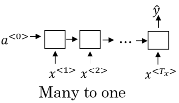
There are different types of network architectures for RNN in terms of how the length of the input relates to the length of the output. A RNN can take a sequence of several tokens as an input and only produce a single value as an output. Such an architecture is called many-to-one and is used for tasks like sentiment analysis where the RNN e.g. tries to predict a movie rating based on a textual description of the critics.

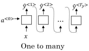
The opposite is also possible: A RNN can take only a single value as input and produce a sequence as an output by re-using the previous outputs to make the next prediction. Such an architecture is called one-to-many. It could be used for example in a RNN that generates music by taking a genre as an input and generates a sequence of notes as an output.

There is theoretically also a one-to-one architecture. However, such an architecture is rarely encountered since it essentially corresponds to a standard NN.

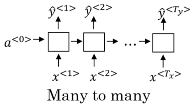
Finally, there are networks which take an input sequence of length $T_x$ and produce an output of length $T_y$. This is called a many-to-many architecture. In the above example, the length of the input was equal to the length of the output. However, input and output sequences need not to be of the same length. This property is especially important for tasks like machine translation where the translated text might be longer or shorter than the original text.

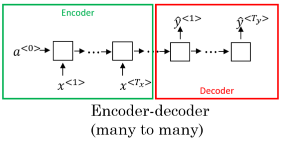
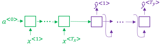
Encoder-Decoder Networks

Models with a many-to-one architecture might be implemented as encoder-decoder models. This is perhaps the most commonly used framework for sequence modelling with neural networks. Like the name suggests, an Encoder-Decoder model consists of two RNNs. The encoder maps the input sequence $X$ to a hidden representation $H$ of the same length as the input. The decoder then consumes this hidden representation to produce $Y$, i.e. make a prediction.

$$H = encode(X) \\ Y=p(Y \vert X) = decode H$$

Language model and sequence generation

RNN can be used for NLP tasks, e.g. in speech recognition to calculate for words that sound the same (homophones) the probability for each writing variant. Such tasks usually require large corpora of text which is tokenized. A token can be a word, a sentence or also just a single character. The most common words could then be kept in a dictionary and vectorized using one-hot encoding. Those word vectors could then be used to represent sentences as a matrix of word vectors. A special vector for the unknown word (<unk>) could be defined for words in a sentece that is not in the dictionary plus an <EOS> vector to indicate the end of a sentence.

The RNN can then calculate in each step the probabilities for each word appearing in the given context using softmax. This means if the dictionary contains the 10’000 most common words the prediction $\hat{y}$ would be a vector of dimensions $(10'000 \times 1$ containing the probabilities for each word. This probabaility is calculate using Bayesian probability given the already seen previous words:

$$\hat{y}^{<t>} = P(x^{<t>} \vert x^{<t-1>}, x^{<t-2>}, ... x^{<1>} )$$

This output vector indicates the probability distribution over all words given a sequence of $t$ words. Predictions can be made until the <EOS> token is processed or until some number of words have been processed. Such a network could be trained with the loss function ($\ref{loss}$) and the cost function ($\ref{cost}$) to predict the next word for a given sequence of words. This also works on character level where the next character is predicted to form a word.

Vanishing Gradients in RNN

Vanishing Gradients are also a problem for RNN. This is especially relevant for language models because a property is that sentences can have relationships between words spanning over a lot of words. Consider the following sequence of tokens representint the sentence The cat, which already ate a lot of food, which was delicious, was full.:

<the> <cat> <which> <already> <ate> <a> <lot> <of> <food> <which> <was> <delicious> <was> <full> <EOS>

Note that the token <was> affects the token <cat>. However, since there are a lot of tokens in between, the RNN will have a hard time predicting the token <was> correctly. To capture long-range dependencies between words the RNN would need to be very deep, which increases the risk of vanishing or exploding gradients. Exploding gradients can relatively easily be solved by using gradient clipping where gradients are clipped to some arbitrary maximal value. Vanishing gradients are harder to deal with and require the use of gated recurrent units (GRU) to memorize words for long range dependencies.

Gated Recurrent Units

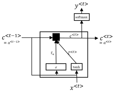
Gated Recurrent Units (GRU) are a modification for the hidden layeres in an RNN that help mitigating the problem of vanishing gradients. GRU are cells in a RNN that have a memory which serves as an additional input to make a prediction. To better understand how GRU cells work, consider the following image depicting how a normal RNN cell works:

Simple GRU

GRU units have a memory cell $c^{<t>}$ to “remember” e.g. that the token <cat> was singular for later time steps. Note that for GRU cells $c^{<t>} = a^{<t>}$ but we still use the variable $c$ for consistency reasons, because in another type of cell (the {LSTM-cell]{#lstm-cells} which will be explained next) we use the same symbol. In each time step a value $\tilde{c}$ is calculated as a candidate to replace the existing content of the memory cell $c$. This candidate uses an activation function (e.g. $\tanh$), its own trainable parameter matrix $W_c$ and a separate bias $b_c$.

$$\begin{equation} \tilde{c}^{<t>} = \tanh \left( W_c \left[ c^{<t-1>}, x^{<t>} \right] + b_c \right) \label{cell_candidate} \end{equation}$$

After calculating the candidate $\tilde{c}^{<t>}$ we use an update-gate $\Gamma_u$ to decide whether we should update the cell with this value or keep the old value. The value for $\Gamma_u$ can be calculated using another trainable parameter matrix $W_u$ and bias $b_u$. Because Sigmoid is used as the activation function, the values for $\Gamma_u$ are always between 0 and 1 (for simplification you can also thing of $\Gamma_u$ to be either exactly 0 or exactly 1).

$$\begin{equation} \Gamma_u = \sigma\left( W_u \left[ c^{<t-1>, x^{<t>}} \right] + b_u \right) \label{update_gate} \end{equation}$$

This gate is the key component of a GRU because it “decides” when to update the memory cell. Combining equations ($\ref{cell_candidate}$) and ($\ref{update_gate}$) gives us the following formula to calculate the value of the memory cell in each time step:

$$\begin{equation} c^{<t>} = \Gamma_u * \tilde{c}^{<t>} + (1 - \Gamma_u) * c^{<t-1>} \label{gru_update} \end{equation}$$

Note that the dimensions of $c^{<t>}$, $\tilde{c}^{<t>}$ and $\Gamma_u$ corresponds to the number of units in the hidden layer. The asterisks $*$ denote element-wise multiplication. The following picture illustrates the calculations inside a GRU cell. The black box stands for the calculations in formula $\ref{gru_update}$.

Full GRU

The above explanations described a simplified version of a GRU with only one gate $\Gamma_u$ to decide whether to update the cell value or not. Because the memory-cell $c$ is a vector with several components you can think of it as a series of bits, whereas each bit remembers one specific feature about the already seen words (e.g. one bit for the fact that <cat> was singular, another bit to remember that the middle sentence was about food etc…). Full GRUs however usually have an additional parameter $\Gamma_r$ that describes the relevance of individual features, which again uses its own parameter matrix $W_r$ and bias $b_r$ to be trained:

$$\begin{equation} \Gamma_r = \sigma\left( W_r \left[ c^{<t-1>, x^{<t>}} \right] + b_r \right) \label{relevance_gate} \end{equation}$$

In short, GRU cells allow a RNN to remember things by using a memory cell which is updated depending on an update-gate $\Gamma_u$. In researach, the symbols used to denote the memory cell $c$, the candidate $\tilde{c}$ and the two gates $\Gamma_u$ and $\Gamma_r$ are sometimes different. The following table contains all the parameters of a full GRU cell including a description and how to calculate them:

Symbol	alternative	Description	Calculation
$\tilde{c}^{<t>}$	$\tilde{h}$	candidate to replace the memory cell value	$\tilde{c}^{<t>} = \tanh\left(W_c \left[ \Gamma_r * c^{<t-1>}, x^{<t>} \right] + b_c \right)$
$\Gamma_u$	$u$	Update-Gate to control whether to update the memory cell or not	$\Gamma_u = \sigma\left( W_u \left[ c^{<t-1>}, x^{<t>} \right] + b_u \right)$
$\Gamma_r$	$r$	Relevance-Gate to control the relevance of the memory cell values for the candidate	$\Gamma_r = \sigma\left( W_r \left[ c^{<t-1>}, x^{<t>} \right] + b_r \right)$
$c^{<t>}$	$h$	new memory cell value at time step $t$	$c^{<t>} = \Gamma_u * \tilde{c}^{<t>} + (1 - \Gamma_u) * c^{<t-1>}$
$a^{<t>}$	-	new activation value	$a^{<t>} = c^{<t>}$

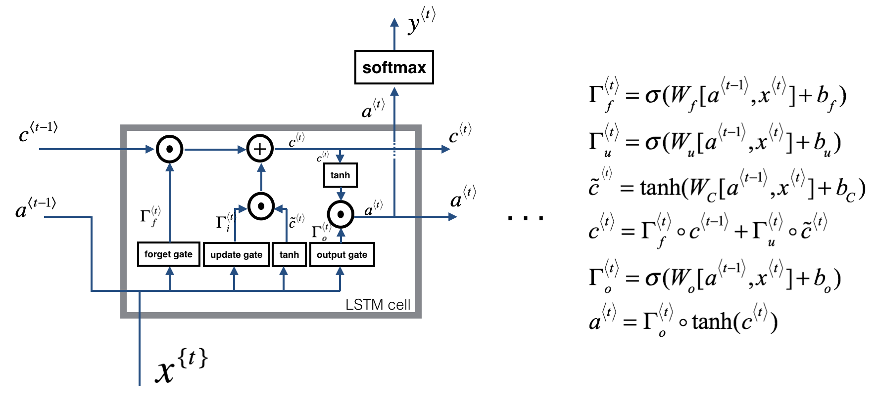
Long Short Term Memory Units

An advanced alternative to GRU are Long Short Term Memory (LSTM) cells. LSTM cells can be considered a more general and more powerful version of GRU cells. Such cells also use a memory cell $c$ to remember something. However, the update of this cell is slightly different from GRU cells.

In contrast to GRU cells, the memory cell does not correspond to the activation value anymore, so for LSTM-cells $c^{<t>} \neq a^{<t>}$. It also does not use a relevance gate $\Gamma_r$ anymore but rather a forget-gate $\Gamma_f$ that governs whether to forget the current cell value or not. Finally, there is a third parameter $\Gamma_o$ to act as output-gate and is used to scale the update memory cell value to calculate the activation value for the next iteration.

The following table summarizes the different parameters and how to calculate them.

Symbol	alternative	Description	Calculation
$\tilde{c}^{<t>}$	$\tilde{h}$	candidate to replace the memory cell value	$\tilde{c}^{<t>} = \tanh\left(W_c \left[ a^{<t-1>}, x^{<t>} \right] + b_c \right)$
$\Gamma_u$	$u$	Update-Gate to control update of memory cell	$\Gamma_u = \sigma\left( W_u \left[ a^{<t-1>}, x^{<t>} \right] + b_u \right)$
$\Gamma_f$	$u$	Forget-Gate to control influence of current memory cell value for the new value	$\Gamma_f = \sigma\left( W_f \left[ a^{<t-1>}, x^{<t>} \right] + b_f \right)$
$\Gamma_o$	$u$	Output-Gate to control influence of current memory cell value for the new value	$\Gamma_o = \sigma\left( W_o \left[ a^{<t-1>}, x^{<t>} \right] + b_o \right)$
$c^{<t>}$	$h$	new memory cell value at time step $t$	$c^{<t>} = \Gamma_u * \tilde{c}^{<t>} + \Gamma_f * c^{<t-1>}$
$a^{<t>}$	-	new activation value	$a^{<t>} = \Gamma_o * \tanh(c^{<t>})$

The following image illustrates how calculations are done in an LSTM cell:

Several of such LSTM cells can be combined to form an LSTM-network. There are variations for the LSTM cell implementation, such as making the gate parameters $\Gamma_u$, $\Gamma_f$ and $\Gamma_o$ not only depend on the previous activation value $a^{<t-1>}$ and the current input token $x^{<t>}$, but also on the previous memory cell valu $c^{<t-1>}$. The update for the update gate is then $\Gamma_u = \sigma\left( W_u \left[ a^{<t-1>}, x^{<t>}, c^{<t-1>} \right] + b_u \right)$ (other gates analogous). This is called a peephole connection.

GRU vs. LSTM

There is not an universal rule when to use GRU- or LSTM-cells. GRU cells represent a simpler model, hence they are more suitable to build a bigger RNN model because they are computationally more efficient and the RNN will scale faster. On the other hand the LSTM-cells are more powerful and more flexible, but they also require more training data. In case of doubt, try LSTM cells because they have sort of become state of the art for RNN.

Bidirectional RNNs

Unidirectional RNNs only consider already seen tokens at a time step $<t>$ to make a prediction. In contrast, bidirectional RNN (BRNN) also take subsequent tokens into account. This is for example helpful for NER when trying to predict whether the word Teddy is part of a name in the following two sencences:

<he> <said> <teddy> <bears> <are> <on> <sale> <EOS>

<he> <said> <teddy> <roosevelt> <was> <a> <great> <president> <EOS>

Just by looking at the previously seen words it is not clear at time step $t=3$ whether <teddy> is part of a name or not. To do that we need the information of the following tokens. A BRNN can do this using an additional layer. During forward propagation the activation values $\overrightarrow{a}$ are computed as seen above from the input tokens and the previous activation values using an RNN cell (normal RNN cell, GRU or LSTM). The second part of forward propagation calculates the values $\overleftarrow{a}$ from left to right using the additional layer. The following picture illustrates this. Note that the arrows in blue and green only indicate the order in which the tokens are evaluated. It does not indicate backpropagation.

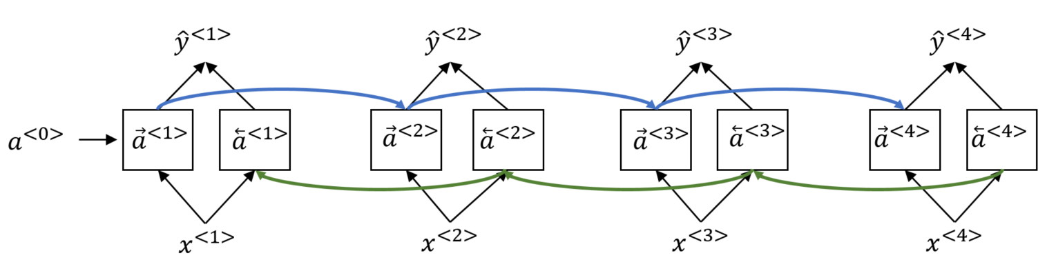
After a single pass of forward propagation a prediction at time step $t$ can be made by stacking the activations of both directions and calculating the prediction value as follows:

$$\hat{y}^{<t>} = g \left( W_y \left[ \overrightarrow{a}^{<t>}, \overleftarrow{a}^{<t>} \right] + b_y \right)$$

The advantage of BRNN is that it allows to take into account words from both directions when making a prediction, which makes it a good fit for many language-related applications like machine translation. On the downside, because tokens from both directions are considered, the whole sequence needs to be processed before a prediction can be made. This makes it unsuitable for tasks like real-time speech recognition.

Deep RNN

The RNNs we have seen so far consisted actually of only one layer (with the exception of the BRNN which used an additional layer for the reverse direction). We can however stack several of those layers on top of each other to get a Deep RNN. In such a network, the results from one layer are passed on to the next layer in each time step $t$:

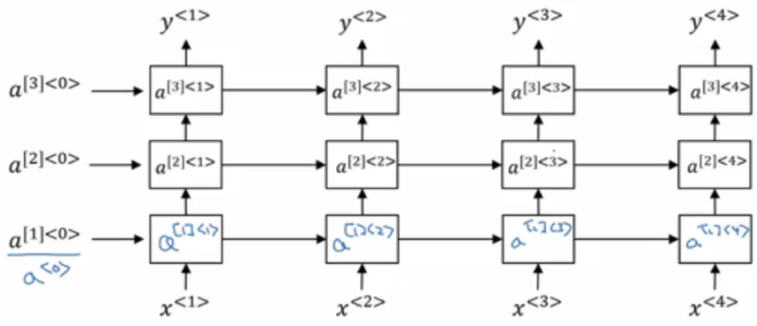
The activation $a^{[l]<t>}$ for layer $l$ at time step $t$ can be calculated as follows:

$$a^{[l]<t>} = g\left( W_a^{[l]} \left[ a^{[l]<t-1>}, a^{[l-1]<t>} \right] + b_a^{[l]}\right)$$

Deep-RNN can become computationally very expensive quickly, therefore they usually do not contain as many stacked layers as we would expect in a conventional Deep-NN.

Natural Language Processing

In the chapter about language modelling above we have seen that we can represent words from a dictionary as vectors using one-hot encoding where all components are zero except for one.

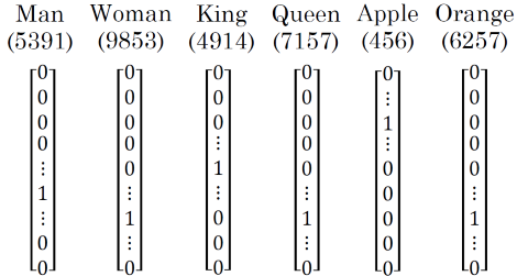
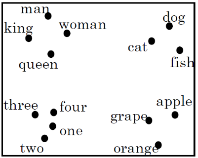
The advantage of such an encoding is that the calculation of a word vector and looking up a word given its vector is easy. On the other hand this form of encoding does not contain any information about the relationships of words between each other. An alternative sort of word vectors are word embeddings. In such vectors, each component of a vector reflects a different feature of a word meaning (e.g. age, sex, food/non-food, word type, etc…). Therefore the components can all have non-null values. Words that are semantically similar have similar values in the individual components. For visualization we could also reduce dimensionality to two (or three) dimensions, e.g. by applying the t-SNE algorithm. By doing so it turns out that words with similar meanings are in similar positions in vector space.

Properties of word embeddings

Word embeddings have become hugely popular in NLP and can for example be used for NER. Oftentimes an existing model can be adjusted for a specific task by performing additional training on suitable training data (transfer learning). This training set and also the dimensionality of the word vectors can be much smaller. The relevance of a word embedding $e$ is simliar to the vector of a face in face recognition in computer vision: It is a vectorized representation of the underlying data. An important distinction however is that in order to get word embeddings a model needs to learn a fixed-size vocabulary. Vectors for words outside this vocabulary can not be calculated. In contrast a CNN could calculate a vector for a face it has never seen before.

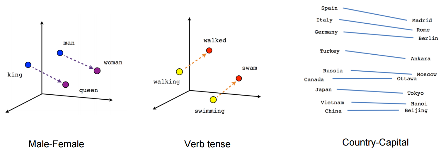
Word embeddings are useful to model analogies and relationships between words. The best known example for this is the one from the original paper:

$$\begin{equation} e_{man} - e_{woman} \approx e_{king} - e_{queen} \label{word2vec_1} \end{equation}$$

The distance between the vectors for “man” and “woman” is similar to the distance between the vectors for “king” and “queen”, because those two pairs of words are related in the same way. We can also observe that a trained model has learned the relationship between these two pairs of words because the vector representations of their distances is approximately parallel. This also applies to other kinds of word pairings, like verbs in different tenses or the relationship between a country and its capital:

Therefore we could get the following equation by rearranging formula $\ref{word2vec_1}$:

$$\begin{equation} e_{king} - e_{man} + e_{woman} \approx e_{queen} \label{word2vec_2} \end{equation}$$

This way the word embedding for “queen” can be calculated using the embeddings of the other words. To get the word for its embedding we can use a similarity function $sim$, which measures the similarity between two embeddings $u$ and $v$. Often the cosine similarity is used for this function:

$$sim(u,v) = \frac{u^T v}{\lVert u\rVert_2 \lVert v \rVert_2}$$

With the help of the similarity function we can find the word for “queen” by comparing the embedding $e_{queen}$ against the embeddings of all other word from the vocabulary:

$$w = \underset{w}{\operatorname{argmax}} sim(e_{queen}, e_{king} - e_{man} + e_{woman})$$

Embedding matrix

The embeddings of the words in the vocabulary can be precomputed and stored in an embedding matrix $*$. This is efficient because the learned embeddings don’t need to be computed each time. The embedding $e_j$ of a word $j$ from the vocabulary can easily be retrieved by multiplying its one-hot encoding $O_j$ with the embedding matrix:

$$\begin{equation} e_j = E \cdot O_j \label{embedding_matrix} \end{equation}$$

However, since most components in $O_j$ are zeroes, a lot of multiplications are done for nothing. Therefore a specialized function is normally used in practice to get the embedding for a word.

Word2Vec

Word2Vec (W2V) is the probably most popular implementation for word embeddings. W2V contains two approaches:

• Skip-Gram
• CBOW (Continuous Bag Of Words)

Skip-Gram

In the skip-gram approach a random word is chosen as context word during training to learn word embeddings. Usually the context words are not chosen with uniform random distribution but according to their frequency in the corpus. Frequent words have a lower probability for being selected as context words. After that a window of e.g. 5 words (i.e. the 5 words before and after) can be defined, from which a target word is sampleed. The learning problem then consists of predicting the target word from the context word, i.e. learning a mapping from the context a the target word.

Consider for example a dictionary of 10’000 words and the two words “orange” (context word) and “juice” (target word, to be learned) as training tuple. For these two words their embeddings $e_c$ and $e_t$ can be retrieved as shown in ($\ref{embedding_matrix}$). The embedding $e_c$ can be fed to a softmax unit which calculates a prediction for the target word embedding $e_t$ as follows:

$$p(t \vert c) = \frac{e^{\Theta^T_t e_c}}{ \sum_{j=1}^{10'000} e^{\Theta^T_j e_c} }$$

The output vector $\hat{y}$ is then a vector with probabilities for all 10’000 words. The training goal should therefore optimize the parameter $\Theta_t$ for the target word so that the probability for $e_t$ (“juice”) is high. The loss function is then as usual the negative log-likelyhood (note that $y$ is the one-hot encoding for the target word, in our example “juice”):

$$\mathcal{L} (\hat{y} ,y) = - \sum_{i=1}^{10'000} y_i \log(\hat{y}_i)$$

Skip-Gram can calculate very good word embeddings. The problem with softmax however is its computational speed. Every time we want to evaluate the probability $p(t \vert c)$ we need to carry out a sum of over all words in the vocabulary. This will not scale well with increasing vocabulary size. To solve this we could apply hieararchical softmax which splits up the computed vector for the cell value by recursively dividing it into halves until the maximum value has been found (divide and conquer).

Negative Sampling

A more performant way of calculating word embeddings is negative sampling, which can be regarded as a modified learning problem than the one used in Skip-Gram. In negative sampling, a training set of $k+1$ samples is created for each valid combination of context and target word by deliberately creating $k$ negative samples.

The learning problem in negative sampling is therefore constructed by creating a pair of words by randomly defining a context word and sampling a target word from a window to get a valid target word. This pair is labelled “1” because it is a valid combination of context and target word. After that, $k$ additional target words are sampled at random from the vocabulary. Those will be labelled “zero” because they are considered non-target words (even if they happen to appear inside the window!). The value for $k$ should be between 5 and 20 for smaller datasets and between 2 and 5 for larger datasets.

This way we get a training set of $k+1$ pairs of words. We can use this to learn a mapping from context to target word by treating the problem as a binary classification problem. In each iteration we train a NN with only these $k+1$ word pairs from the dataset (in contrast to Skip-Gram where the training is done over the whole vocabulary). The probability an arbitrary target word $t'$ and the context word $$c$ co-occurring is defined as follows:

$$P(y=1 \vert c,t') = \sigma (\Theta_c^T e_c)$$

The learning problem is therefore to reduce the parameters $\Theta_c$ so that the cost is minimal (i.e. $P(y=1 \vert c,t) \approx 1$).

GloVe

An alternative to W2V is GloVe, which (although not as popular as W2V) has some advantages over W2V due to its simplicity. The GloVe algorithm counts for a given word $i$ the co-occurrence of each other word $j$ in a certain context. The notion of context can be defined arbitrarily, e.g. by defining a window like in Skip-Gram. This means for each word $j$ a value $x_{ij}$ is calculated.

The learning problem is then defined by minimizing the following function (again for a vocabulary of 10’000 words):

$$\begin{equation} minimize \sum_{i=1}^{10'000} \sum_{j=1}^{10'000} f(x_{ij}) (\Theta_i^T e_j + b_i + b'_j - \log x_{ij})^2 \label{glove_min} \end{equation}$$

The function $f(x_{ij})$ calculates a weighting term for the individual values of $x_{ij}$ with the following properties:

• If $x_{ij}=0$ (word $j$ does not co-occur with word $i$ then $f(x_{ij}) = 0$. This prevents the above formulat to calculate $\log(x_{ij}) = \infty$. In other words: by multiplying with $f(x_{ij})$ we only sum up the values of $x_{ij}$ for pairs of words that actually co-occur at least once.
• more frequent words get a higher weight than less frequent words. At the same time the weight is not too large to prevent stop-words from having too much influence.
• less frequent words get a smaller weight than more frequent words. At the same time the weight is not too small so that even rare words have some sensible influence.

With this learning problem the terms $\Theta_i$ and $e_j$ are symmetric, i.e. they end up with the same optimization objective. Therefore the embedding for a given word $w$ can be calculated by taking the average of $e_w$ and $\Theta_w$.

It turns out that even with such a simple function to minimize as seen in ($\ref{glove_min}$) good word embeddings can be learned. This simplicity compared to W2V is somewhat surprising and might be a reason for GloVe to be popular for some researchers.

Sentiment classification

Sentiment classification (SC) is the process of deciding from a text whether the writer likes or dislikes something. This is for example required to map textual reviews to star-ratings (1 star=bad, 5 stars=great).

The learning problem in SC is to learn a function which maps an input $x$ (e.g. a restaurant review) to a discrete output $y$ (e.g. a star-rating). Therefore the learning problem is a multinomial classification problem where the predicted class is the number of stars. For such learning problems, however, training data is usually sparse.

A simple classifier could consist of calculating the word embeddings for each word in the review and calculating their average. This average vector could then be fed into a softmax classifier which calculates the probability for each of the target classes. This also works for long reviews because the average vector will always have the same dimensionality. However, by averaging the word vectors we lose information about the order of the words. This is important because the word sequence “not good” should have a negative impact on the star-rating whereas when calculating the average of “not” and “good” individually the negative meaning is lost and the star-rating would be influenced positively. An alternative would therefore be to train an RNN with the word embeddings.

Debiasing Word Embeddings

Word Embeddings can suffer from bias depending on the training data used. The term bias denotes bias towards gender/race/age/etc… here, not the numeric value often seen before. Such stereotypes can become a problem because they can enforce stereotypes by learning inappropriate relationship between words (e.g. man is to computer programmer as woman is to homemaker). To neutralize such biases, you could perform the following steps:

1. Identify bias direction: If for example we want to reduce the gender bias we could define pairs of male and female forms of words and average the difference between their embeddings (e.g. $frac{e_{he} - e_{she}}{2}$). The resulting vector gives us the bias direction $g$.
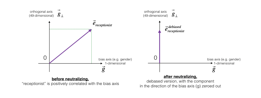
2. Neutralize: For every word that is not definitional, project to get rid of bias. Definitional means that the gender is important for the meaning of the word. An example for a definitional word is grandmother or grandfather, because here the gender information cannot be omitted without losing semantic meaning. We can compute the neutralized embedding as follows:

$$e^{bias\_component} = \frac{e \cdot g}{||g||_2^2} * g \\ e^{debiased} = e - e^{bias\_component}$$

The figure below should help you visualize what neutralizing does. If you’re using a 50-dimensional word embedding, the 50 dimensional space can be split into two parts: The bias-direction $g$ , and the remaining 49 dimensions, which we’ll call $g_{\perp}$. In linear algebra, we say that the 49 dimensional $g_{\perp}$ is perpendicular (or “othogonal”) to $g_{\perp}$, meaning it is at 90 degrees to gg . The neutralization step takes a vector such as $e_{receptionist}$ and zeros out the component in the direction of gg , giving us $e_{receptionist}^{debiased}$ . Even though $g_{\perp}$ is 49 dimensional, given the limitations of what we can draw on a screen, we illustrate it using a 1 dimensional axis below.

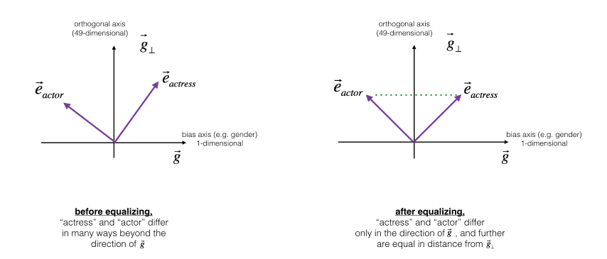
1. Equalize pairs: Equalization is applied to pairs of words that you might want to have differ only through the gender property. As a concrete example, suppose that “actress” is closer to “babysit” than “actor.” By applying neutralizing to “babysit” we can reduce the gender-stereotype associated with babysitting. But this still does not guarantee that “actor” and “actress” are equidistant from “babysit.” The equalization algorithm takes care of this. The key idea behind equalization is to make sure that a particular pair of words are equi-distant from the 49-dimensional $g_\perp$. The equalization step also ensures that the two equalized steps are now the same distance from $e_{receptionist}^{debiased}$, or from any other work that has been neutralized. In pictures, this is how equalization works:

In the above steps we used gender bias as an example, but the same steps can be applied to eliminate other types of bias too. Word embedding will almost alway suffer from bias that is intrinsically contained in the corpora they wore learned from.

Sequence-to-sequence models

We have learned that RNNs with a many-to-many architecture (with encode-decoder networks as a special form) take a sequence as an input and also produce a sequence as their output. Such models are called Sequence-to-Sequence (S2S) models. Such networks are traditionally used in machine translation where the input consists of sentences, which are transformed by an encoder network to serve as the input for the decoder network which does the actual translation. The output is then again a sequence, namely the translated sentence. The same process works likewise for other data. You could for instance take an image as an image as input and have an RNN try to produce a sentence that states what is on the picture (image captioning). The encoder network in this case could then be a conventional CNN whereas the last layer will contain the image as a vector. This vector is then served to an RNN which acts as the decoder network to make predictions. Assuming you have enough already captioned images as training data an RNN could then learn how to produce captions for yet unseen images.

S2S in machine translation

There area certain similarities between S2S-models and the previously seen language-models where we had an RNN produce a sequence of words based on the probability of previously seen words in the sequence:

In such a setting the output was generated by producing a somewhat random sequence of words. However, that is not what we want in machine translation. Here we usually want the most likely sentence that corresponds to the best translation for a given input sentence. This is a key difference between language models as seen before and machine translation models. So in contrast to the model above, a machine translation model does not start with the zero vector as the first token, but rather takes a whole sentence and encodes it using the encoder part of the network.

In that respect one can think of a machine translation model as kind of conditional language model that calculates the probability of a translated sentence given the input sentence in the original language.

Beam search

Suppose we have the following french sentence as an input:

Jane visite l'Afrique en septembre.

Possible translations to English for this sentence could be:

• Jane is visiting Africa in September.
• Jane is going to be visiting Africa in September.
• In September, Jane will visit Africa.
• Her African friend welcomed Jane in September.

Each of these sentences is a more or less adequate translation of the input sentence. One possible approach to calculate the most likely sentence (i.e. the best translation) is going through the words one by one to calculate the joint probability of a sentence by always taking the most probable word in each step as the next token. This approach is called greedy search and although it is fairly simple, it does not work well for machine translation. This is because small differences in probability for earlier words can have a big impact on what sentence is picked after inspection of all tokens. By using greedy search we would also try to find the best translation in a set of exponentially many sentences. Considering a vocabulary of 10’000 words and a sentence length of 10 words this would yield a solution space of $$10'000^{10}$ theoretically possible sentences.

Another approach which works reasonably well is beam search (BS). BS is an approximative approach, i.e. it tries to find a good enough solution. This has computational advantages over exact approaches like BFS or DFS, meaning the algorithm runs much faster but does not guarantee to find the exact optimum.

BS also goes through the sequence of words one by one. But instead of choosing the one most likely word as the next token in each step, it considers a number of alternatives. This number $B$ is called the beam width. In each step, only the $B$ most likely choices are kept as the next word. This means that a partial sequance is not further evaluated if it does not continue with one of the $B$ most likely words. The following figure illustrates this:

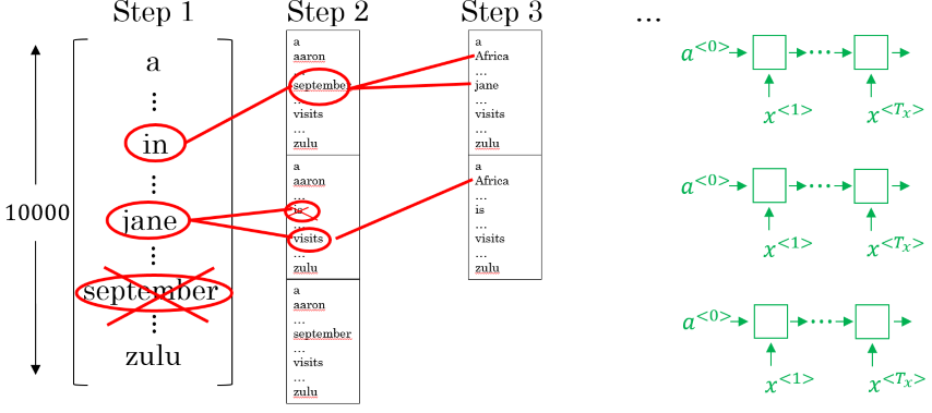
The higher the value for $B$ the more alternatives are considered in each step, hence the more combinatorial paths are followed and the computationally more expensive the algorithm becomes. With a value of $B=1$ BS essentially becomes greedy search. Productive systems usually choose a value between 10 and 100 for $B$. Larger values like $1000 < B < 3000$ happen to be used for research purposes, although the final utility will decrease the bigger $B$ becomes.

Refinements to Beam Search

There are a few tricks that help improving BS performance- or result-wise:

• Length normalization
• Error analysis

Length normalization

We have seen BS maximizing the following probability:

$$\begin{align*} \arg \max & \prod_{t=1}^{T_y} P(y^{<t>} \vert x, y^{<1>}, ..., y^{<t-1>} ) \\ & = P(y^{<1>}, ..., y^{<T_y>} \vert x ) \\ & = P(y^{<1>} \vert x) \cdot P(y^{<2>} \vert x, y^{<1>}) \cdot ... \cdot P(y^{<T_y>} \vert x, y^{<1>}, ..., y^{<T_y - 1>}) \end{align*}$$

The problem with this is that the probabilities of the individual tokens are usually much smaller than 1 which results in an overall probability which might be too small to be stored by a computer (numerical underflow). Therefore, the following formula is used to keep the calculation numerically more stable and less prone to rounding errors:

$$\arg \max \sum_{y=1}^{T_y} \log P(y^{<t>} \vert x, y^{<1>}, ..., y^{<T_y -1>})$$

Because the logarithm is a strictly monotonically increasing function maximizing the product of probabilities is the same as maximizing the sum of their logarithms. However, this formula will still result in shorter sequences because the overall probability for a sentence will only decrease the longer it gets. Longer sequences are therefore penalized while shorter sequences benefit from the higher probability. To fix this, a normalization parameter $\alpha$ is introduced and the term is normalized by dividing by a power of the number of words in the sequence (length normalization):

$$\arg \max \frac{1}{T_y^\alpha} \sum_{y=1}^{T_y} \log P(y^{<t>} \vert x, y^{<1>}, ..., y^{<T_y -1>})$$

The hyperparamter $\alpha$ controls the degree of normalization. This means instead of comparing the raw values for the probability of a partial sequence, Beam Search will compare the normalized values. For values of $\alpha \rightarrow 1$ the term is completely normalized, for values of $\alpha \rightarrow 0$ no normalization is done.

Error Analysis

If a system does not output sequences with the desired quality we have to examine where causes for this are possibly rooted: in the RNN model itself or in the Beam Search algorithm.

Consider the French sentence “Jane visite l’Afrique en septembre” from above. We now compare this sentence to the following sentences:

• $y^*$: optimal translation by a humen (e.g. “Jane visits Africa in September.”
• $\hat{y}$: translation from the model (e.g. “Jane visited Africa last September.”

In this example it is evident that the model did not output a good translation. We can now distinguish the following cases for the probabilities of those two sentences (from the set of all possible sentences).

• $P(y^* \vert x > P(\hat{y} \vert x)$: In this case the algorithm chose the sentence with the lower probability. The cause for the error is therefore rooted in the search algorithm (Beam Search).
• $P(y^* \vert x \leq P(\hat{y} \vert x)$: In this case the algorithm calculated a too small probability for the optimal translation. The cause for the error is therefore rooted in the model (RNN).

To get a feeling for where most errors are rooted we could make this comparison for a number of samples and analyze where most errors are rooted.

Bleu Score

A special property of translation is that there are possibly many different translation which are considered equally correct. Since linguistics is not an exact science and language itself is somewhat fuzzy due to its ambiguousity, the evaluation of NLP tasks naturally contains a grey area where the distinction between correct or wrong is not clear.

One method to compare two texts (e.g. human and machine translation) is to calculate the Bleu-Score (Bilingual evaluation understudy). This value measures the quality of a translation as degree of overlap with a (or several) reference translation(s). A higher value means a better quality.

The Bleu score therefore measures the precision as the number of words in the translation that also appear in the reference. Note that to calculate recall we could use Rouge. Consider the following translations for the French sentence “Le chat es sur le tapis.”

Reference translation 1	The cat is on the mat.
Reference translation 2	There is a cat on the mat.
Translation	the the the the the the the (7 words)

Because the word the appears in at least one of the reference translation, the resulting Bleu-score would be $\frac{7}{7} = 1$ (i.e. a perfect translation). However, this is obviously wrong. Therefore a modified precision is used which limits the number of counted appearances to the maximum number of appearances in either one of the sentences. Because in the above example the word the appears twice in the first reference translation and once in the second reference translation, this maximum is 2 and the modified precision is therefore $\frac{2}{7}$.

Instead of looking at words in isolation (unigrams) we could also look at pairs of words (bigrams), triplets (3-grams) or generally tuples of any number. For this the machine translation sentence is split into its different bigrams which are then counted. We could then additionally calculate a clip count which indicates in how many of the reference sentences the bigram appears.

Bigram	Count	Clip Count
the cat	2	1
cat the	1	0
cat on	1	1
on the	1	1
the mat	1	1

The modified n-gram-precision could then be calculated by dividing the sum of clipped counts by the sum of all counts:

$$p_n = \frac{\sum_{\text{n-gram} \in \hat{y}} count_{clip}(\text{n-gram})} {\sum_{\text{n-gram} \in \hat{y}} count(\text{n-gram})}$$

For the above example, the $p_2$ value would be $\frac{4}{6} \approx 0.666$. A good translation has values for different n-grams close to 1. All n-gram-scores can be combined to the combined Bleu score:

$$\exp \left( \frac{1}{4} \sum_{n=1}^4 p_n \right)$$

Of course, again short translations have an advantage here because there are fewer possibilities for errors. An extreme example of this would be a translation in form of a single word which would get a score of 1 if only this words appears in the reference translations. To prevent this, an adjustment factor called brevity penalty (BP) is introduced, which penalizes short translations:

$$BP = \begin{cases} 1 & \text{if lenghts are equal}\\ \exp\left( 1 - \frac{ \text{machine translation}_{\text{length}} }{ \text{reference translation}_{\text{length}} } \right) & otherwise \end{cases}$$

Attention models

So far the task of machine translation has only been exemplified with sequence models following an encoder-decoder-architecture where one RNN “reads” a sentence and encodes it as a vector and another RNN makes the translation. This works well for comparatively short sentences. However, for long sentences the performance (e.g. measured by Bleu score) will decrease. This is because instead start translating a very long sentence chunk by chunk (like a human would) it is difficult to make an RNN memorize the whole sentece because it is processed all in one go.

A modification to the encoder-decoder-architecture are attention models (AM). AM process a sentence similarly to how a human would by splitting it up into several chunks (contexts) of equal size and translating each chunk separately. This is especially useful in tasks with real-time requirements like speech recognition or simultaneous translation where you usually don’t want to wait for the whole input to be available before making a prediction. For each context $c$ the model computes the amount attention it should pay to each word. The output for this chunk serves as input for the next chunk.

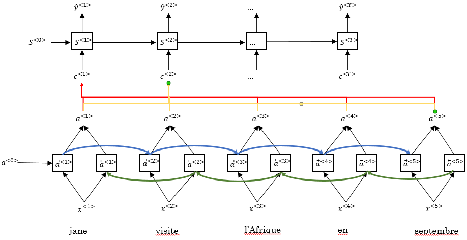
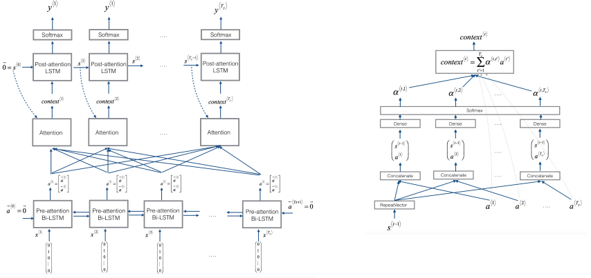
As an example consider the chunk “Jane visite l’Afrique en septembre…” from a much longer French sentence. This chunk of tokens $x^{<t'>}$ is being processed by a bidirectional RNN which acts as an encoder-network by encoding the chunk as set of features $a^{<t'>} = (\overrightarrow{a}^{<t'>}, \overleftarrow{a}^{<t'>})$ (one feature per word). Note that $t'$ denotes the time step for the current chunk whereas $t$ denotes the time step over the whole sequence.

Those features are then weighted by weights $\alpha^{<t, t'>}$ which must sum up to 1. Those weights indicate how much attention the model should pay to the specific feature (therefore the term attention model). The weighted features are then summed up to form a context $c^{<t>}$. A different context is calculated for each time step $t$ with different weights. All the contexts are then processed by an unidirectional decoder-RNN which makes the actual predictions $\hat{y}^{<t>}$

The attention weights can be learned as follows:

$$\begin{equation} \alpha^{<t,t'>} = \frac{ \exp( e^{<t,t'>} ) } { \sum_{t'=1}^{T_x} \exp( e^{<t,t'>} ) } \label{attention_model_e} \end{equation}$$

Note that the above formula $\ref{attention_model_e}$ only makes the attention weights sum up to 1. The actual attention weights are in the parameter $e$, which is a trainable parameter that is learned by the decoder network, which can be trained by a very small neural network itself:

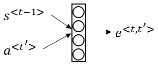
The figure below shows an example for an attention model as well as the calculation of the attention weights inside a single step.

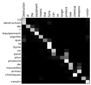
The magnitude of the different attentions during processing can further be visualized:

To sum up, here are the most important parameters in an attention model

Symbol	description	calculation
$a^{<t'>}$	feature for the decoder network at chunk-timestep $t'$	$a^{<t'>} = (\overrightarrow{a}^{<t'>}, \overleftarrow{a}^{<t'>})$
$\alpha^{<t,t'>}$	amount of attention $\hat{y}^{<t>}$ should pay to chunk-feature $a^{<t'>}$ at time step $t$ ($\sum_{t'} \alpha^{<t,t'>} = 1$)	$\alpha^{<t,t'>} = \frac{\exp( e^{<t,t'>} ) }{ \sum_{t'=1}^{T_x} \exp( e^{<t,t'>} ) }$
$c^{<t>}$	context for the decoder network at time step $t$	$c^{<t>} = \sum_{t'} \alpha^{<t,t'>} a^{<t'>}$
$\hat{y}^{<t>}$	prediction of decoder network at time step $t$

The advantage of an attention model is that it does not process individual words one by one, but rather pays different degrees of attention to different parts of a sentence during processing. This makes them a good fit for tasks like machine translation or image captioning. On the downside the model takes quadratic time to train because for $T_x$ input tokens and $T_y$ output tokens the number of trainable parameters is $T_x\cdot T_y$ (i.e. it has quadratic cost).

If you want to know more about Attention Models, there is a wonderful explanation on Distill.

Speech recognition

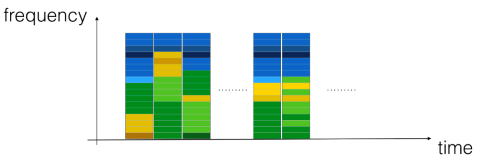
The problem in speech recognition is that there is usually much more input than output data. Take for example the sentence “The quick brown fox jumps over the lazy dog.” which consists of 35 letters. An audio clip of a recording of this sentence which 10s length and was recorded with a sampling rate of 100Hz (100 samples per second) however has 1000 input samples! The samples of an audio clip can be visualized using a spectrogram.

Traditional approaches to get the transcription for a piece of audio involved aligning individual sounds (phonemes) with the audio signal. For this, a phonetic transcription of the text using the International Phonetic alphabet (IPA) was needed. The alignment process then involved detecting individual phonemes in the audio signal and matching them up with the phonetic transcription. To do this, Hidden Markov Models (HMM) were often used. This method was state of the art for a long time, however it requires an exact phonetic transcription of the speech and is prone to features of the audio signal (e.g. sampling rate, background noise, number of speakers), the text being spoken (intonation, pronunciation, language, speaking rate) or the speaker itself (pitch of the voice, gender, accent).

A more recent approach for speech recognition is a technique called Connectionist Temporal Classification (CTC). In contrast to HMM, CTC does not need an exact phonetic transcription of the speech audio (i.e. it is alignment-free). The CTC method allows for directly transforming an input signal using an RNN. This is constrasting to the HMM approach where the transcript first had to be mapped to a phonetic translation and the audio signal was then mapped to the individual phonemes. The whole process allows the RNN to output a sequence of characters that is much shorter than the sequence of input tokens.

The underlying principle of CTC is that the input (i.e. spectrograms) are each mapped not only to a single character, but to all characters of the alphabet at the same time (with different probabilities). This may output in a sequence of characters like this:

ttt_h_eee_____ _____q___...

This process usually generates a whole bunch of possible output sequences, which can then be further reduced by passing it through a CTC-cost function, which collapses repeated characters. By doing this, we get a set of possible transcriptions, which can then be evaluated by means of a language model, which yields the most likely sequence to form the transcript for the audio.

The main advantage of CTC is that it not only outpeforms all previous models but also that it does not require an intermediate phonetic transcription (i.e. it is an end-to-end model). If you want to know more about CTC, read the original paper or pay a visit to this wonderful explanation ond Distill.

Trigger word detection

A special application of speech recognition is trigger word detection, where the focus lies on detecting certain words inside an audio signal to trigger some action. Such systems are widely used in mobile phones or home speakers to wake up the device and make it listen to further instructions.

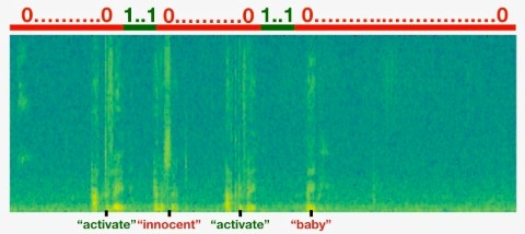
To train such a system the label for the signal can be simplified by marking it as 0 for time slots where the trigger word is not being said an 1 right after the trigger word was said. Usually a row of ones are used to prevent the amount of zeros being overly large and also because the end of the trigger word might not be easy to define exactly.

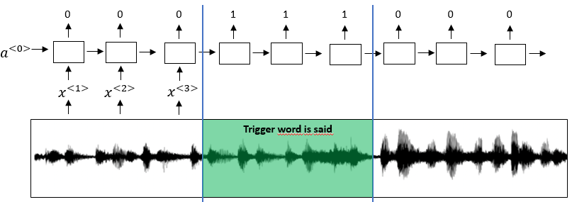
The labelling of input data in trigger word detection can also be illustrated by visualizing the audio clip’s spectrogram together with the $y$-labels. The following figure contains the spectrogram of an audio clip containing the words “innocent” and “baby” as well as the activation word “activate”.