Table of Contents

• Course overview
• Hyperparameter tuning
• Training-, Validation- and Test-Set
  • Bias and variance
• Regularization
  • Regularizing the cost
    • Regularization term for NN
    • Adjusting parameter update
    • Why adding the regularization term reduces overfitting
  • Dropout
  • Other regularization techniques
    • Data augmentation
    • Early stopping
• Input normalization
• Initialization
• Model Optimization
  • Mini Batch Gradient Descent
    • Understanding MBGD
  • Exponentially weighted average
  • Momentum
  • RMSprop
  • Adam
  • Learning Rate decay
• Hyperparameter tuning
• Batch Normalization
  • Why does BN work?
• Multiclass classification

Course overview

Week 1 introduces the various hyperparameters of a model and how to choose reasonable values for them. You will also learn how to identify problematic behavior of algorithm and where it may be rooted. Week 2 introduces some optimization algorithms that may speed up the overall learning process. Week 3 wraps up on hyperparameters and how to find optimal values for them. It also introduces Softmax as an alternative activation function for multiclass-classification. This is also the week where you get to know a DL-Framework (TensorFlow) for the first time.

Hyperparameter tuning

We have learned in part 1 that setting up a NN is a highly iterative and empirical process. There is no algorithm that can calculate the optimal values for the hyperparameters (e.g. number of layers, hidden units or learning rate) for you. Sometimes there are a few rule of thumbs you can use. But more often the values for the hyperparameters are chosen more or less intuitively.

It is also true that results from one domain can seldom be transferred to another. So if you have a NN that works well in computer vision, it is not guaranteed that this NN also works well for audio or language processing tasks. Most of the time it is impossible to “guess” the optimal values in the first try. They have to be manually adjusted to improve learning. This requires experience which can be obtained through practice - or by someone who tells you what works (and what not). And this is exactly what this course is aimed at.

Training-, Validation- and Test-Set

The available labelled data is usually split into three parts:

Name	Purpose	Ratio
training set	for the actual training of the model	>90%
validation set (sometimes also called dev-set)	for parameter optimization	<5%
test set	for modelevaluation	<5%

In earlier years of ML a usual split was 60/20/20% (training/test/validation). You can sometimes still see these numbers in textbooks. This split was valid for times when labelled data was scarce and you had to make sure to have enough instances in your validation or test set. However, for a lot of DL tasks nowadays there is enough data available, so we can use a lot bigger portion for training while optimizing/testing with a comparatively small validation/test set. The suggested ratios in the table above apply to scenarios where a lot of training data is available. This is kind of a precondition for DL models in order to achieve a good performance. However, we live in an imperfect world and labelled data might still not always be readily available. In such situations your split ratios may vary in favor of a larger validation and/or training set. It really depends on your specific setting.

The reason we split into different set is that we can optimize the model by using data it has never seen before. We do this to reduce overfitting. We can later evaluate the model with another set of instances it has - again - never seen before and therefore get a realistic sense for how the model will perform in the real world for unseen data.

If not much labelled data is available, people sometimes use only a training and a test set and then optimize their model by using the test set. In fact, this is sometimes done regardless of the amount of labelled data. But be aware: this is actually wrong! If you optimize your model on your test set, your model has (implicitly) already seen this data (indirectly, through optimization) and you’re left with no more unseen data to evaluate your model on. When evaluating your model with the same test data you used for optimizing the parameters the results might be too optimistic!

Bias and variance

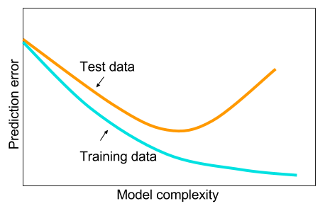
A well known problem in ML is overfitting. Overfitting means you trained your model applies very wellon the training data but does not generalize well for unseen data. In contrast, you can also train your model too little. We then speak of underfitting. The following image shows typical graphs for the error on the training set and the error on the test set with a model that is overfitting. Notice how the error on the training and test data decrease up to some point when the error on the test data starts to increase again. That’s the point when your model starts to overfit!

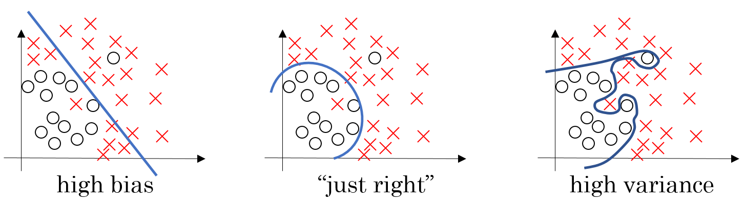
In context of over- or underfitting there are two other terms often used: bias and variance. We speak of high bias when your model is underfitting, i.e. it is not trained enough and biased too much towards the training data. In contrast, we speak of high variance if your model is trying too hard and is therefore overfitting. The following picture visualizes how a model with high bias or high variance might classify the instances:

The following table shows the different combinations of high/low bias and variance and what they mean (train set error means your cost on the training set and dev-set error means the error when optimizing on the dev set):

	dev-set error high	DevSet error low
train set error high	high bias and variance	you got lucky (unrealistic case)
train set error low	high bias	your model performs well

If your model suffers of high bias, you could train a bigger network, train longer (i.e. more iterations) or choose a different architecture. If your model suffers of high variance you should try to get more training data or apply some of the regularization techniques presented below.

To assess the quality of a model the difference between bias and variance is relevant. Generally, we try to keep this difference as small as possible.

Regularization

We can prevent overfitting by applying one or more regularization techniques which are presented in this chapter.

Regularizing the cost

A common approach for regularization is to add a regularization term to the cost function. For example, we can add regularize the cost function for Logistic Regression when optimizing the parameters $w$ and $b$:

$$\require{color} \begin{equation} J(w,b) = \frac{1}{m} \sum_{i=1}^m \mathcal{L}(\hat{y}^{(i)}, y^{(i)}) \colorbox{yellow} {$ + \frac{\lambda}{2m} \lVert w \rVert^2_2 $} \label{regularization_lr} \end{equation}$$

The last term $\frac{\lambda}{2m}\ \lVert w \rVert^2_2$ is called the regularization term and uses the regularization hyperparameter $\lambda$, which determines the degree of the regularization. In this case, we use $\lVert w \rVert^2_2$ in the regularization term, which is called the L2-norm and is defined as follows:

$$\lVert w \rVert^2_2 = \sum_{j=1}^{n_x} w_j^2 = w^Tw$$

However, we could also use the L1-norm which is less common but would be defined as follows:

$$\lVert w \rVert_1 = \sum_{j=1}^{n_x} \vert w_j \vert$$

Regularization term for NN

We have seen now how we can regularize the cost in Logistic Regression by using a regularization term (see $\ref{regularization_lr}$). We can regularize the cost in a NN with several hidden layers (and therefore several weight matrices $W^{[l]}$) the same way using a similar regularization term:

$$\require{color} \begin{equation} J(W^{[1]},b^{[1]}, ..., W^{[l]},b^{[l]}) = \frac{1}{m} \sum_{i=1}^m \mathcal{L}(\hat{y}^{(i)}, y^{(i)}) \colorbox{yellow} {$ + \frac{\lambda}{2m} \sum_{l=1}^L \lVert W^{[l]} \rVert^2_F $} \label{regularization_nn} \end{equation}$$

Note that the term $\lVert W^{[l]} \rVert^2_F$ is basically just the L2-norm, but is often called the Frobenius norm for historical reasons. It calculates the values by iterating over the rows and columns of a weight matrix $W^{[l]}$ for Layer $l$ with dimension $(n^{[l]} \times n^{[l-1]})$ and is defined as follows::

$$\lVert W^{[l]} \rVert^2_F = \sum_{i=1}^{n^{[l]}} \sum_{j=1}^{n^{[l-1]}} (w_{ij}^{[l]})^2$$

So adding a regularization term to the cost function leads to higher costs. Therefore high values in $W$ are penalized when calculating the cost. Note that the bias parameter $b$ is usually not regularized. This is because $W$ is usually a high dimensional matrix with lots of values and $b$ just a scalar, so regularizing $b$ won’t make much of a difference.

Adjusting parameter update

Because we changed the calculation of the cost by using a regularization term, we also need to adjust the derivative when updating the weights:

$$\begin{equation} \require{color} dW^{[l]} = \frac{\partial J}{\partial W^{[l]}} = \textit{\{value from backprop\}} \colorbox{yellow}{$ + \frac{\lambda}{m} W^{[l]} $} \\ \rightarrow W^{[l]} = W^{[l]} - \alpha dW^{[l]} \label{regularization_parameter_update} \end{equation}$$

Re-writing the above equation $\ref{regularization_parameter_update}$ a bit gives us the following equation:

$$\begin{align*} W^{[l]} & = W^{[l]} - \alpha dW^{[l]} \\ & = W^{[l]} - \alpha ( \textit{\{value from backprop\}} + \frac{\lambda}{m} W^{[l]} ) \\ & = W^{[l]} - \frac{\alpha\lambda}{m} W^{[l]} - \alpha(\textit{\{value from backprop\}}) \\ & = (1 - \frac{\alpha\lambda}{m}) W^{[l]} - \alpha(\textit{\{value from backprop\}}) \end{align*}$$

We see in the last form that the weight matrix $W^{[l]}$ is multiplied with $(1 - \frac{\alpha\lambda}{m})$, which is a value smaller than one. Cosequently, the values of the weight matrix become a bit smaller in each iteration. That’s why L2-Regularization in NN is sometimes also referred to as weight decay.

Why adding the regularization term reduces overfitting

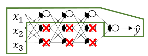
The reason why a regularization term leads to a better model is that with weight decay single weights in a weight matrix can become very small. The weight matrix is then in fact a sparse matrix. This leads to single nodes virtually being cancelled out in the NN and effectively to a simpler NN.

Another reason is that the activation function $g$ is roughly linear for values close to zero. We can observe this when using $tanh$ as our activation function:

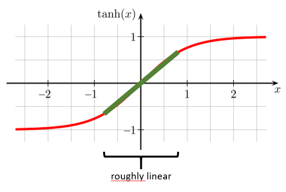
Because the values in $W^{[l]}$ become close to zero, the cell value $Z^{[l]} = W^{[l]} a^{[l-1]} + b^{[l]}$ (before activation) is also close to zero. Therefore, the values after activation mostly lie in the linear region of the activation function. Therefore the NN calculates something more or less close to a linear function. As we have seen in part one, linear classifiers can only calculate linear boundaries. Therefore the higher the value for $\lambda$ the more we force the NN to become close to a linear function and prevent it to calculate over-complicated boundaries. This consequently reduces overfitting.

Dropout

Another technique to reduce overfitting is using Dropouts. With dropouts we mean completely cancelling out individual neurons during test time by multiplying their weights by zero. By doing this we prevent single neurons in the NN to become too important for learning. In other words: We force the NN to learn from other features too. To make this work, we must cancel out different units in each iteration during training time. When doing this, the ratio of cancelled out neurons in each layer should not be more than 50%. Dropout regularization works surprisingly well for certain domains such as computer vision. On the downside we can’t really rely on the costs calculated by $J$ anymore because different units are cancelled out in each iteration. To get around this you should plot your costs without and then with dropout regularization to make sure they are really decreasing. Important: during test time we mustn’t use dropout regularization anymore because we want to see the performance of the full network!

Other regularization techniques

Minimizing the costs and preventing overfitting should be treated as separate tasks. This principle is also referred to as orthogonalization. There are several other techniques you can try to reduce overfitting.

Data augmentation

The most common approach to reduce overfitting is to use more training data. But sometimes it is impossible or very expensive to get additional labelled data. We then can try to generate new synthetic data from the old. If we e.g. train an image classifier, we can easily generate new images from the old by applying one or more of the following operations:

• mirroring
• rotation
• random cropping
• shifting
• tilting
• local warping / adding some noise
• color shifting

There are tools and libraries to help with data augmentation (e.g. Agumentor for image data). However, this can only be done to some extent because the underlying image information is factually still the same and using more of “the same” will not improve the model significantly anymore at some point.

Early stopping

Another very simple method to prevent overfitting is to abort training as soon as we observe the test error increasing again. However, this is problematic because we prevent the model from exploring the whole label space. It also violates the principle of orthogonalization.

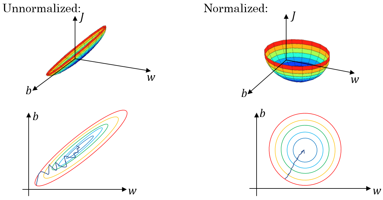
Input normalization

A very useful technique to speed up the learning process is to normalize the NN’s input. We can do this in two steps:

• subtract the mean: $\mu = \frac{1}{m} \sum_{i=1}^m x^{(i)} \\ x = x - \mu$
• divide by the variance: $\sigma^2 = \frac{1}{m} \sum_{i=1}^m {x^{(i)}}^2 \\ x = \frac{x}{\sigma}^2$

Subtracting the mean will center the values around their average value, meaning that samples with feature values close to the mean vector will have values close to zero. Dividing by the variance will put the feature values on a similar scale, meaning that big differences between values in skewed data will be reduced. Normalizing the inputs leads to the cost function converging more quickly. However, when performing input normalization this way you should make sure to use the same values for $\mu$ and $\sigma$ to normalize the training and the test set!

Initialization

The problem with very deep NN is that for each layer $l$ we have a weight matrix $W^{[l]}$ with values that can be big (greater than 1) or small (less than 1). Because each layer multiplies the previous layer’s activation with its own weight matrix, this can lead to very high or very small values for $\hat{y}$. This applies if all (or a lot) of the weight matrices contain big values and consequently the value for $\hat{y}$ exponentially increases/decreases. A similar argument can be used to show that also the gradients will exonentially increase/decrease (exploding or vanishing gradients).

A partial solution for this problem is a careful initialization of the parameters for the NN. To better understand this let’s observe the following example of a single neuron:

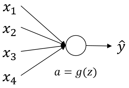
Calculating the cell state $z$ is done as follows:

$$z = w^T x = w_1x_1 + w_2x_2 + ... + w_nx_n$$

To prevent $z$ from becoming very large we have to make sure the single summands don’t become too large. We can do this by multiplying the weight matrix with its variance:

$$W^{[l]} = W^{[l]} \cdot \sqrt{\frac{2}{n^{[l-1]}})}$$

This variant is called He initialization is often used in conjunction with a ReLU activation function. There are other variants for other activation functions, such as Xavier initialization for $tanh$ activation function:

$$W^{[l]} = W^{[l]} \cdot \sqrt{\frac{1}{n^{[l-1]}}}$$

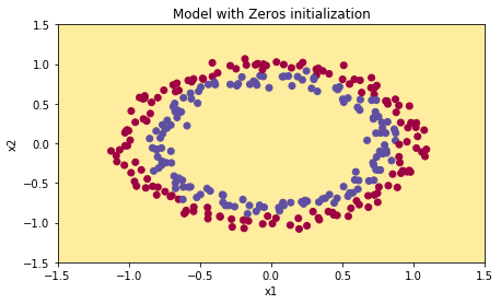
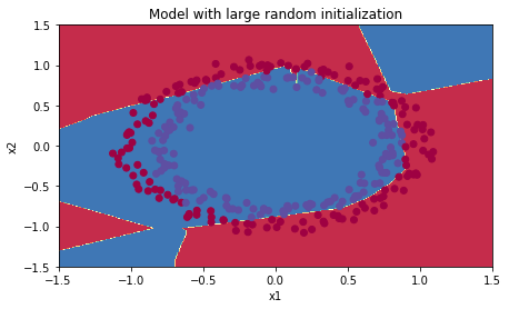
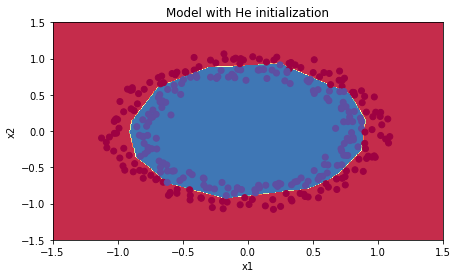
The following picture illustrate the different results for different initializations. Note that for zero-initialization the classifier predicted $0$ (does not belong to class) for all instances!

Model Optimization

It is often hard to find the best model because model training is time-intensive and it can therefore take some time before you get some feedback. To speed up the training process there are a few algorithms.

Mini Batch Gradient Descent

We have learned in part one how vectorization can reduce computation time because all the samples are processed in one go. However, this does not work well for very large datasets anymore because the sample matrix $X$ would simply become too large. We can therefore partition the training set in mini batches, which are processed one by one. Usually, the training data is shuffled prior to partitioning to get randomized batches.

We can identify an individual batch from a set of $T$ batches by adding the superscript $\{t\}$. The processing per batch is than as before for the whole training set:

1. forward-propagation: $A^{[l]} = g(W^{[l]} X^{\{t\}} + b^{\{t\}})$
2. calculate costs: $J^{\{t\}} = \frac{1}{T} \sum_{i=1}^l \mathcal{L} (\hat{y}^{(i)}, y^{(i)}) + \frac{\lambda}{2T} \sum_l \lVert W^{[l]} \rVert^2_F$
3. backprop to compute gradients w.r.t. $J^{\{t\}}$
4. parameter update: $W^{[l]} = W^{[l]} - \alpha dW^{[l]} \\ b^{[l]} = b^{[l]} - \alpha db^{[l]}$

You can see that in fact we are doing exactly the same thing as before, but with a single batch $(X^{\{t\}}, Y^{\{t\}})$ instead of the whole training set. A single iteration over all batches of the training set is called epoch. Like before, training one the whole training set is done with more than 1 iteration. You can thereefore think of MBGD as nesting the existing loop for the training in an additional loop over the batches.

Understanding MBGD

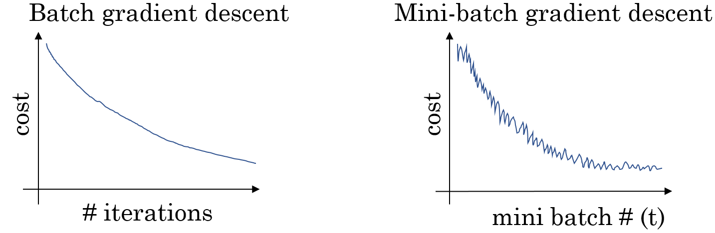
Despite having an additional loop, training with MBGD is usually much faster than processing all the training data at once. Because the batches contain different samples, it is very likely that the costs will not always monotonically decrease from one batch to the next. They usually oscillate a bit, but generally the costs go down:

There are two extrema for choosing the size $s$ of a single mini-batch:

• $s=m$: This corresponds to normal Gradient Descent whereas each training sample is processed individually. This is not recommended because one epoch would take too long.
• $s=1$: This is called stochastic Gradient Descent, which is sometimes done, but we lose the performance advantage of a vectorized implementation

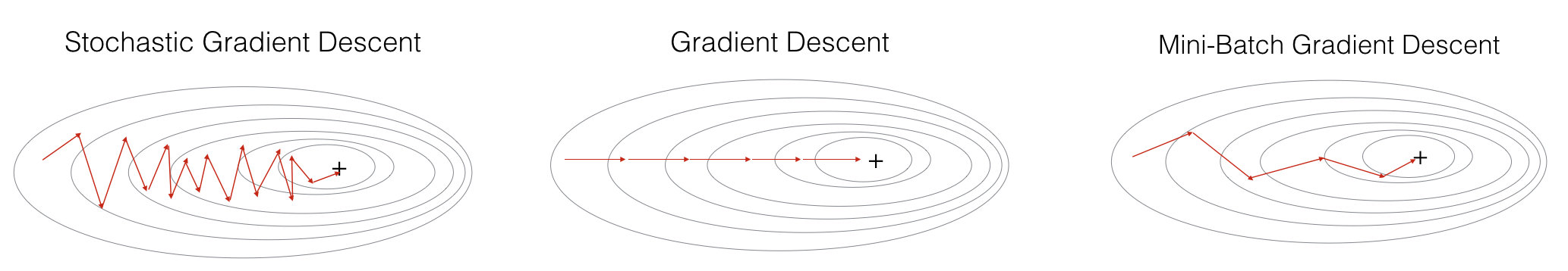
Generally you should choose a value between 1 and $m$ for $s$. Powers of 2 (64, 128, 256, …) are often chosen because they offer some computational advantages. But more important is that a single mini-batch fits into your computer’s memory.

Exponentially weighted average

There are more sophisticated optimization algorithms than GD. They often make use of something called exponentially weighted (moving) average. An EWA $v_t$ can be calculated by recursively by using the previous average $v_{t-1}$, a parameter $\beta$ and the current parameter value $\Theta$:

$$\begin{equation} v_t = \beta v_{t-1} + (1 - \beta) \Theta_t \label{ewa} \end{equation}$$

For example consider the following plot of temperatures over different days (blue dots).

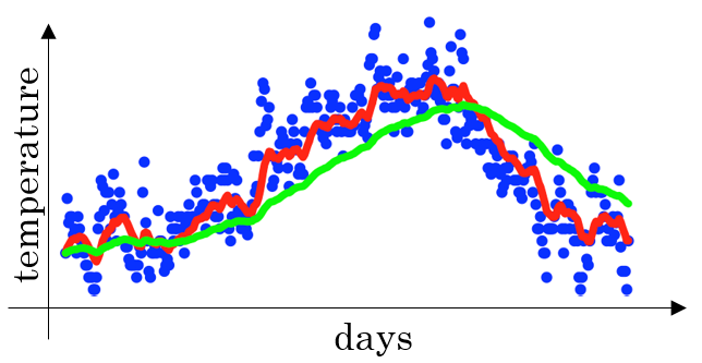
The parameter $\beta$ can here be somehow seen as the window size that is used to calculate the approximate average. A value of $\beta=0.9$ would correspond to $\frac{1}{1-\beta} = 10$ days (red line). A larger value of $\beta = 0.98$ would lead to a larger window of 50 days and consequently to a smoother line, which adapts more slowly to temperature changes and is therefore shifted to the right (green line). In contrast, a smaller value for $\beta$ would consider fewer days and be more wiggly.

When implementing the EWA and initializing $v_0 = 0$ you can observe that the graph of the EWA is too small because the value for the first average is too low. To come around this, one can simply divide the calculated average by $(1-\beta^t)$. This is called bias correction. So formula $\ref{ewa}$ can be adjusted as follows:

$$\begin{equation} v_t = \frac{\beta v_{t-1} + (1 - \beta) \Theta_t}{1-\beta^t} \label{ewa_bias_correction} \end{equation}$$

Momentum

Gradient Descent with momentum (GDM) is a variant of GD which converges faster by using moving averages. GDM can be best understood by observing the convergence of the cost function over a contour plot:

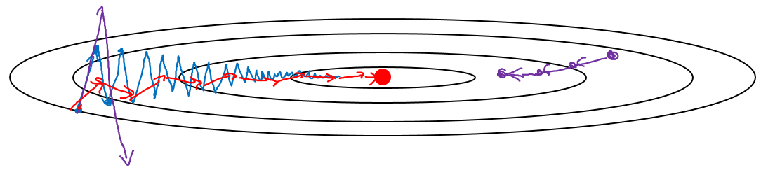
In this figure convergence without GM would follow the blue line, which oscillates quite a bit. This oscillation prevents us from choosing a larger learning rate, because then we would overshoot and maybe even diverge from the optimal costs (purple line). What we want is the oscillation in vertical direction (e.g. the direction for parameter $b$) to damp out because it slows down the learning progress. On the other hand we want learning to go fast in the horizontal direction (e.g. the direction for parameter $W$). By computing the moving averages over the derivatives $dW$ and $db$ GDM smoothes out the steps of GD by cancelling out positive and negative values of the GD (which are responsible for the oscillation in the first place). This makes the GD being more directed towards the optimum and using fewer steps.

So what GDM tries to do is use the learning rate’s momentum for faster convergence in horizontal direction. You can think of the plot above as the contours of a bowl where we roll a ball to its bottom. The averages $v_{dW}/v_{db}$ is responsible for its velocity, and the derivatives $dW/db$ for its acceleration. GDM tries to do this by using a parameter $\beta$. To better understand this, remember how we updated the parameters in GD:

$$W = W - \alpha dW \\ b = b - \alpha db$$

GDM calculates the EWA of the derivatives first and then uses the result to update the parameters:

$$\begin{equation} v_{dW} = \beta v_{dW} + (1 - \beta) dW \\ v_{db} = \beta v_{db} + (1 - \beta) db \\ W = W - \alpha v_{dW} \\ b = b - \alpha v_{db} \label{gdm} \end{equation}$$

Note that bias correction is not usually done in practice because after a few iterations the moving average will have moved up enough to produce good values.

RMSprop

Another algorithm to increase learning speed that makes use of momentum is Root Mean Square prop (RMSprop). The calculation is similiar to GDM (see $\ref{gdm}$), however the derivatives are squared (element-wise) and the update is a bit different.

$$\begin{equation} s_{dW} = \beta s_{dW} + (1 - \beta) dW^2 \\ s_{db} = \beta s_{db} + (1 - \beta) db^2 \\ W = W - \alpha \frac{dW}{\sqrt{s_{dW}} + \epsilon} \\ b = b - \alpha \frac{db}{\sqrt{s_{db}} + \epsilon} \\ \label{rmsprop} \end{equation}$$

Note that the parameter $\epsilon$ is used to prevent division by zero.

In contrast to GDM, RMSprop tries to damp out the vertical oscillation. In other words, for equation $\ref{rmsprop}$ we want $s_{dW}$ to be small, because then we would divide by a small number, which results in a bigger update. On the other hand we expect $s_{db}$ to be large, because then we divide by a large number which would make the update small.

Adam

It turned out over time that a lot of optimization algorithms do not generalize well. Often a certain algorithm only performs well for one specific type of problem. Adaptive Moment Estimation (ADAM) is one of the few algorithms that can be applied to a wide range of learning problems. ADAM is a combination of both GDM and RMSprop. In order to not confuse the differet parameters we will use $\beta_1$ for the parameter of GDM and $\beta_2$ for the parameter of RMSprop. The algorithm can then calculate Gradient Descent for a given mini-batch as follows:

• Initialization: $v_{dW}=s_{dW}=v_{db}=s_{db}=0$
• For each mini-batch in iteration $t$ do:
  • calculate the derivatives $dW, db$
  • calculate moving average with GDM: use $\beta_1$ to determine the window size $v_{dW} = \beta_1 v_{dW} + (1-\beta_1) dW \\ v_{db} = \beta_1 v_{db} + (1-\beta_1) db$
  • calculate RMSprop: use $\beta_2$ to determine damping $s_{dW} = \beta_2 s_{dW} + (1-\beta_2) dW^2 \\ s_{db} = \beta_2 s_{db} + (1-\beta_2) db^2$
  • apply bias correction: $v_{dW} = \frac{v_{dW}}{1-\beta_1^t }, v_{db} = \frac{v_{db}}{1-\beta_1^t } \\ s_{dW} = \frac{s_{dW}}{1-\beta_1^t }, s_{db} = \frac{s_{db}}{1-\beta_1^t }$
  • update parameters: $W = W - \alpha \frac{v_{dW}}{\sqrt{s_{dW}} + \epsilon}, b = b - \alpha \frac{v_{db}}{\sqrt{s_{db}} + \epsilon}$

To sum up, ADAM uses the following hyperparameters:

hyperparameter	meaning	comment
$\alpha$	learning rate	needs to be manually tuned (but ADAM allows for bigger values than GD!)
$\beta_1$	window size to calculate moving average of $dW, db$ (first moment)	0.9 is a reasonable value
$\beta_2$	damping rate to calculate moving average of $dW^2, db^2$ (second moment)	0.999 is a reasonable value
$\epsilon$	term to prevent division by zero	is usually not tuned, but $10^{-8}$ is a reasonable value

Learning Rate decay

It can sometimes make sense to keep the learning rate large at the beginning and then gradually reduce it the more the algorithm converges towards the optimum. This process is called learning rate decay (LRD). The reason LRD can make sense is that during the initial steps of optimization the algorithm can take larger steps whereas at the end it should take only small steps in order to oscillate within a smaller region around the optimum.

To implement LRD the learning rate $\alpha$ starts out with an initial value $\alpha_0$ and is then reduced after each epoch by calculating:

$$\alpha = \frac{1}{1 + \text{\{decay rate\}} \cdot \text{\{#epoch\}}} \cdot \alpha_0$$

There are variations on this, for example:

• $\alpha = \text{\{decay rate\}}^{\text{\{#epoch\}}} \cdot \alpha_0$ (exponential decay)
• $\frac{k}{ \sqrt{ \text{\{#epoch\}} } }$ or $\frac{k}{ \sqrt{t} }$ ($k$ is a constant hyperparameter, $t$ is the number of the mini-batch)
• stepwise reduction after a few steps (discrete decay)
• manual decay: might work when only training a small number of models

Hyperparameter tuning

Until now we have seen quite a lot of hyperparmeters (learning rate $\alpha$, number of layers, number of hidden units, learning rate decay, …). Trying out all possible combinations of these would be infeasible. It also would not make much sense to try out all different combinations, because some of the parameters are more important than others thus a lot of meaningless combinations would also be tried. In practice you usually start out with random values and see where there are regions of values that produce good results. Some of the hyperparameters like the number of layers or hidden units could actually be systematically tried out using grid search, if they are normally distributed. For other parameters like the learning rate it makes most sense only to search in the interval $[0.0001, 0.1]$. This is epsecially important for parameters like $\beta$ that are more sensitive (i.e. small changes on them can have a high impact on the performance of an algorithm). Such parameters should periodically be re-evaluated to see if the original intuition is still justified.

When tuning hyperparameters, there are generally two paradigms:

• Pandas: Only train one model on which you continuously fine-tune its hyperparameters. This is often done if computational power is scarce.
• Caviar: Train several models simultaneously and evaluate them. This is usually done if there is a lot of computational power available

These terms are derived from zoology because pandas usually have only one cub whereas sturgeons produce a lot of eggs (caviar).

Batch Normalization

We have seen that normalizing the input can lead to faster learning in the individual units. We can do this for any hidden layer by performing the following steps:

• Compute the mean of layer $l$:

$$\mu = \frac{1}{m} \sum_i z^{[l](i)}$$

• Compute the variance of layer $l$:

$$\sigma^2 = \frac{1}{m} \sum_i (z^{[l](i)} - \mu )^2$$

• Compute the layer norm:

$$z_{norm}^{[l](i)} = \frac{z^{[l](i)} - \mu}{\sqrt{\sigma^2 + \epsilon}}$$

• Compute the batch norm:

$$\tilde{z}^{[l](i)} = \gamma \cdot z_{norm}^{[l](i)} + \beta$$

There is some debate whether to normalize the cell values before ($z$) or after activation ($a$). In practice, the former is more common. The parameters $\gamma$ and $\beta$ are learnable and can be different for each layer. They allow the mean and variance of $\tilde{z}^{[l](i)}$ to any value. For example, choosing $\gamma = \sqrt{\sigma^2 + \epsilon}$ and $\beta = \mu$ would lead to the same value as before normalization (identity function):

$$\begin{align*} \tilde{z}^{[l](i)} & = \gamma \cdot z_{norm}^{[l](i)} + \beta \\ & = \gamma \cdot \frac{z^{[l](i)} - \mu}{\sqrt{\sigma^2 + \epsilon}} + \beta \\ & = \sqrt{\sigma^2 + \epsilon} \cdot \frac{z^{[l](i)} - \mu}{\sqrt{\sigma^2 + \epsilon}} + \mu \\ & = z_{norm}^{[l](i)} \end{align*}$$

Using BN can lead to a much more robust NN, a broader range of possible hyperparameters and easier training of deep NN. BN is implemented in most common DL-Frameworks like TensorFlow or Keras. Most of the time you don’t have to fiddle with $\gamma$ and $\beta$. However, if you want to adjust the mean and/or variaince of your batch norm explicitly (i.e. to make use of some specific region of your activation function), there are parameters to do exactly that.

Why does BN work?

BN can improve the learning process dramatically. The reason for this is BN reduces the degree, to which input values for a given hidden layers vary (known as covariant shift, because mean and variance always lie within a certain region.

(to be extended)

Multiclass classification

Up to know we have only talked about binary classifiers. The output layer in these NN consisted of a single neuron whose Sigmoid activation function output the probability of an instance belonging to the target class (or not). However, we often have more than one target class, i.e. NN with more than one neuron.

In such networks we distinguish $C$ classes, i.e. $n^{[L]} = C$, whereas each node indicates the probability of an instance belonging to a specific class. We can then use an activation function which is known as softmax which calculates the activation of this output layer as follows:

• calculate vector $t$ by element-wise exponentiation

$$t = e^{z^{[L]}}$$

• calculatae the activation $a^{[L]}$ by dividing $t$ by the sum of its elements:

$$a^{[L]} = \frac{e^{z^{[L]}}}{ \sum_{j=1}^C t_i }$$

In contrast to the other activations (Sigmoid, Tanh, …) softmax is a function from vector to vector. The sum of all elements in the activation value is 1. The term softmax indicates the classifier’s ability to express membership of an instance with a class not just binary but by probability. In that respect, sigmoid is kind of a special form of softmax for only two classes.