Table of Contents

• Course Overview
• Introduction to Deep Learning
• Logistic Regression as a NN
• Designing a NN from scratch
  • Defining the neural network structure
  • Initializing the parameters
  • Forward propagation
  • Computing the loss
  • Computing the gradient with backpropagation
  • Updating the parameters
  • Putting it all together
  • Making predictions on unknown instances
• Shallow Neural Networks
  • Random initialization
• Deep Neural Networks
• Activation functions

Course Overview

The first week focuses on theoretical aspects, different types of NN and possible appliances. There is no programming assignment in this week yet. In the second week you will learn how to see Logistic Regression with one unit as the simplest form of a neural network. You will learn what an activation function is and why you should use one. You will do two programming assignments. The first one is an (optional) introduction to Numpy and vectorization, which you can skip if you are already familiar with this module. If not, you should do this assignment and maybe even invest a bit more time on those technologies using extracurricular tutorials because Numpy is a very common Python module for ML. In the second assignment you will implement logistic regression “bare metal”, i.e. by just using Python and Numpy. The third week will introduce shallow neural networks, i.e. NN with one hidden layer. You will get to know alternative activation functions. You will see how forward- and backpropagation can be implemented in a vectorized manner as well as why parameters should be initialized randomly. In the programming assignment you will implement a first “real” NN, although it only has one hidden layer (i.e. not a Deep-NN). Finally in week four you will implement your first Deep-NN step by step. The network will be used in a follow-up assignment for a binary classifier that can recognize cat pictures with fairly high accuracy. You can even test it with your own pictures!

Introduction to Deep Learning

Deep Learning has really become a household name in recent years because the methods and techniques outperformed a lot of what was state of the art before. A lot of problems became solvable or learnable by means of Neural Networks - especially but not limited to Computer Vision, Audio Processing, language/translation tasks, and so on. NN became really popular when they undercut then-standard algorithms on unstructured data (images, audio, text). It is sometimes forgotten that NN can also be applied on structured data, too. A possible cause for the sudden hype of NN is twofold:

• computational power has seen a dramatic increase over the past 10-20 years
• huge loads of data have become readily available with digitalization (particularly the advent of the internet and mobile devices)

The reason, why NN usually dominate over traditional ML algorithms (SVM, Logistic Regression, …) today is that NN usually become better the more data is available. In contrast, traditional methods usually reach a certain point from which they can only improve marginally, regardless of how much data is available. That’s why we speak about training a NN. However, more complex tasks require more training data (“Scale drives deep learning progress”). The performance of NN is possibly only limited by the available data and computational power. On the other hand, if only little data is available, traditional methods might still outperform NN even today. How much data is enough for a given task, however, is an active field of research.

So Neural Networks (NN) are at the core of what Deep Learning is. NN can be used in supervised or unsupervised learning settings, although I think they are still more often applied in the former while unsupervised learning is often referred to as the holy grail of ML. One can roughly distinguish the following NN types:

• Deep-NN (NN): This is the standard form of a NN and can be seen as a prototype for other variations of NN. This part is all about Deep-NN.
• Convolutional Neural Networks (CNN): These networks are often used for Computer Vision task (image recognition, image classification, …). You can read about them in part 4 of this article series.
• Recurrent Neural Networks (RNN): These networks are often used for one-dimensional, sequential data such as speech/audio, text and so on. You can read about them in part 5 about sequence models

There’s a zoo of other forms and combinations of NN, like Generative Adversarial Networks (GAN), Variational Autoencoders (VAE) and many more, which have gained momentum in the past years. However, I only know them conceptually and will refrain therefore of including them in this list (for now).

Logistic Regression as a NN

As seen in Andrew’s introductory course in ML a binary classification problem can be solved with Logistic Regression (LR). By observing features $x=(x_1, x_2, ..., x_n)$ we try to predict whether a given sample instance $x^{(i)}$ belongs to a certain class or not. This can be visualized by treating the features as coordinates, plotting the sample instances as points and then drawing a line that optimally separates these points into two groups or classes (of course this kind of visualization only makes sense when there’s not more than two or three features, because we can’t plot in more than three dimensions):

(example image here)

To fit the line optimally we usually take a bunch of labelled sample instances (i.e. samples where we know the class already). Such a training instance can be represented by the tuple $(x,y)$, where $x$ is said feature vector and $y$ either the number zero (instance does not belong to class) or one (instance belongs to class). Logistic Regression tries to approximate the separating line so that the overall error of all training instances is minimal. After the optimal parameters to separate the training instances have been learned, the same parameters can be applied to unlabeled (unknown) instances to decide whether a given instance belongs to the class or not. This can be done by calculating the probability that a single instance belongs to the class. An unlabelled instance can be represented by the tuple $(x,\hat{y})$, whereas $x$ is again a feature vector and $\hat{y}$ the probability $P(y=1 \vert x)$ that the instance belongs to the class (given $x$).

To define what “optimal” means we need a loss function that tells us big the discrepancy between the prediction ($\hat{y}^{(i)}$) and the actual class ($y^{(i)}$) is for a single training sample. Note that $y^{(i)}$ refers to the label for the $i$-th trainings sample. Generally, you can choose whatever loss function you like, for example the Mean Squared Error function, which is defined as follows:

$$\mathcal{L}(\hat{y}^{(i)}, y^{(i)}) = \frac{1}{2}(\hat{y}^{(i)} - y^{(i)})^2$$

In linear regression however the Log Loss Function is used for logistic regression:

$$\begin{equation} \mathcal{L}(\hat{y}^{(i)}, y^{(i)}) = - y^{(i)} \log(\hat{y}^{(i)}) - (1-y^{(i)} ) \log(1-\hat{y}^{(i)}) \label{loss} \end{equation}$$

The cost function calculates the average loss (i.e. cost) over all $m$ training instances classified with the current parameters:

$$\begin{equation} J=\frac{1}{m} \sum_{i=1}^m(\mathcal{L}y^{(i)}, \hat{y}^{(i)}) \label{cost} \end{equation}$$

Designing a NN from scratch

Let’s say for example that we want to predict housing prices by observing the features of a set of known houses where we already know the price. The features of an individual house taken into account might be its size, number of bedrooms, zip code, wealth of the neighborhood and so on. Those features must be transformed into a numeric representation somehow in order to be used as a feature vector. We can then train above NN. The general methodology to build a NN is usually as follows (we will describe the unknown terms below):

1. Define a neural network architecture: number of input units, number of hidden units, number of layers, etc…
2. Initialize the model’s parameters
3. Loop
4. implement forward propagation
5. compute loss
6. implement backward propagation to get the gradients
7. update the parameters with gradient descent

This process is usually iterative, empirical process in that we try to find the optimal hyperparameters (e.g. network architecture) by trial and error. We will learn some tricks to make this a guided process in part 2.

Defining the neural network structure

For now, let’s assume we stick with the simplest NN model with only one layer containing a single unit. This unit is the output unit, receiving the input from an input layer to whom it is connected. So the number of hidden layers is 0 (zero). Let’s now further assume we observe $n$ features. A single feature vector can therefore be defined with an $(n \times 1)$ vector. If we stack the feature vectors of all $m$ training examples we get a training matrix $M$ with dimensions $(n \times m)$ Smiliarly, we have the labels of all trainings samples, which are either $0$ or $1$. We can stack those and get a label vector $y$ of dimensions $(1 \times m)$ Because we only have a single node and we try to fit a straight line between the points, we only have two parameters to optimize: the weights for the individual features (giving us the slope of the line) and the bias (giving us the y-intersect or threshold). We can represent the weights as an $(n \times 1)$ vector $(w_1, w_2)$ and the bias as a scaler $b$. To sum up, we have now the following parameters:

Symbol	Meaning	Dimensions
$n$	number of features	scalar
$m$	number of training samples	scalar
$X$	training sample matrix (one feature vector per training sample)	$(n \times m)$
$y$	training label vector	$(1 \times m)$
$w$	weight vector (one weight per feature)	$(n \times 1)$
$b$	bias (threshold)	scalar
$\Theta$	parameter matrix containing the weights and the bias (one row with weight and bias per feature)	$(n \times 2)$

Initializing the parameters

Because we do not know the optimal parameters from the beginning, we need to initialize them to reasonable values and then optimize them through training. So let’s initialize the parameters $w$ and $b$ with zeroes. We will see later, why that’s not a good idea for Deep-NN, but for a NN with only one node this works. We now have $b=0$ and $w=(0, 0)$.

Forward propagation

We can now compute the cell state $z^{(i)}$ for a given sample instance $x^{(i)}$ by calculating: $z^{(i)}=w^T x^{(i)} + b$

This cell state needs to go through an activation function first before it can be used for classification. We will see later why we need an activation function and what activation functions there are. For now, let’s just use the Sigmoid function which is defined as:

$$\begin{equation} \sigma (z)=\frac{1}{z + e^{-z}} \label{sigmoid} \end{equation}$$

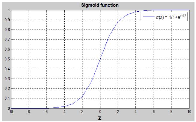
This function produces only values within the interval $[0,1]$. If $z$ is a large positive number, then $\sigma (z) \approx 1$. If $z$ is a small or large negative number, then $\sigma (z) \approx 1$. If $z=0$ then $\sigma (z) = 0.5$ By putting the cell state through the activation function we get the activation $a^{(i)} = \hat{y}^{(i)}=\sigma(z^{(i)})=\sigma(w^T x^{(i)} + b)$ of the neuron. We can do this for all training samples simultaneously by computing:

$$A=\sigma (w^T X + b)$$

Computing the loss

According to the formulas for the loss ($\ref{loss}$) and the cost ($\ref{cost}$) we can now compute the cost for the current iteration over all training samples as follows (note that $a^{(i)}=\sigma(w^T x^{(i)} + b)$ refers to the activation of the neuron for the $i$-th training sample):

$$J=-\frac{1}{m} \sum_{i=1}^m(y\log(a^{(i)}) + (1 - y)\log(1 - a^{(i)}))$$

Computing the gradient with backpropagation

We can calculate the partial derivative as follows:

$$dw = \frac{\partial J}{\partial w}=\frac{1}{m}X(A-Y)^T$$ $$db = \frac{\partial J}{\partial b}=\frac{1}{m}\sum_{i=1}^m(a^{(i)}-y^{(i)})$$

Updating the parameters

To update the parameters Gradient Descent GD is commonly used. We can choose a fixed learning rate $\alpha$ arbitrarily. However, choosing this value wisely is crucial: if it is too big, we might never reach the optimal values, because GD will “overshoot” it. If we choose $\alpha$ too small, GD might be very slow. The following animations illustrate this.

value for $\alpha$ is reasonable	$\alpha$ is too large

We learn more on it in part 2 about hyperparameter tuning. For now let’s assume we chose a reasonable value for $\alpha$ and can therefore update the parameters as follows:

$$\Theta=\Theta - \alpha d\Theta$$

Putting it all together

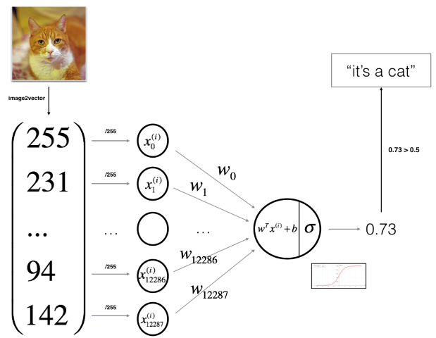
We have seen that by Logistic Regression we try find the parameters $w$ and $b$ that minimize the overall cost $J$. A NN can perform Logistic regression exactly the same way. In fact, traditional binary Logistic Regression can be seen as a NN in its simplest form: with only one single neuron (a.k.a. unit or cell) and therefore only two parameters to learn. For instance, if we want to build a classifier that classifies images into cat pictures ($y=1$) or no cat pictures ($y=0$). We can unroll the image’s pixels into a feature vector, where each feature corresponds to the RGB-value of an individual pixel. I.e. if the image is 64x64 pixels, we get $64 \cdot 64\cdot 3=12288$ features. The one-neuron NN is then as follows:

Making predictions on unknown instances

Having found our optimal values for $\Theta$ we can now predict the membership of unknown instances by their probability. To calculate the probability we simply compute forward propagation again with the optimized $\Theta$ and the sample’s feature vector.

$$\sigma (w^T x^{(i)} + b)= \begin{cases} \ge 0.5 & x^{(i)} \text{ belongs to class}\\ < 0.5 & x^{(i)} \text{ does not belong to class} \end{cases}$$

Shallow Neural Networks

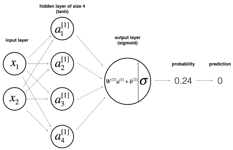
The explanations above were made for a single neuron. However, we can now expand this example to a NN using a hidden layer with several neurons and apply the sampe principles. We still have a single neuron as the output layer. A shallow NN with two features (i.e. two neurons in the input layer), one hidden layer and a single neuron in the output layer (i.e. binary classification) might therefore look like this:

The only change we make is that instead of a weight vector $w$ we now use a weight matrix $W^{[i]}$ holding the weights for each neuron in the layer $i$. Since we have The computations are then as follows (similar to the equations for a single neuron):

$$Z^{[1]}=W^{[1]} X + b^{[1]} \\ A^{[1]}=\sigma(Z^{[1]}) \\ Z^{[2]}=W^{[2]} X + b^{[2]} \\ A^{[2]}=\sigma(Z^{[2]})$$

Or more generally:

$$\begin{equation} A^{[i]}=\sigma(W^{[i]} X + b^{[i]}) \label{forwardprop} \end{equation}$$

Random initialization

When using a single neuron for logistic we have initialized the parameters $w$ and $b$ with zeroes. This does not work for NN with more than one neuron anymore. The reason for this is that if the weights and biases were all initialized with zeroes, every node in the layer would compute exactly the same thing in forward propagation. Consequently, the gradients in backprop would also be the same. Of course this is not what we want. We want every neuron to compute something different. For that reason it is important to initialize the weights with random values. There are different variations of how this could be done, for example Xavier-Initialization or He-Initialization. Most frameworks like TensorFlow or Keras readily provide implementations for these variations.

Deep Neural Networks

We started with a single neuron for Logistic Regression. We expanded this example to a shallow NN with one hidden layer containing several neurons. We can now take this further and construct a deep NN with several hidden layers.

Activation functions

You might have wondered why we used an activation function (the Sigmoid-function $\sigma$) at all. Why couldn’t we just take the cell state $Z^{[i]}$? Well, we could do this, but then the end result in the output layer would be the combination of several linear functions ($W^{[i]} X + b^{[i]}$, see $\ref{forwardprop}$), which is itself a linear combination. The NN would then not be better than Logistic Regression. So the goal of using an activation function is to break linearity.

Apart from the Sigmoid-Function there are several other activation functions. To name the most common:

Name	Definition	Description
Tanh	$a= \frac{e^z-e^{-z}}{e^z+e^{-z}}$	Similar to Sigmoid, but the values are in the interval $[-1, 1]$
ReLU (Rectified Linear Unit)	$a=max(0,z)$	The derivatives of this function are not defined for $z=0$, but this does not matter in practice
Leaky ReLU	$a=max(0.01z,z)$	The coefficient $0.01$ is arbitrary and could be chosen greater/smaller. However, this value is often used in practice