Table of Contents

• Course overview
• CNN in computer vision
  • Convolution by example
  • Padding
  • Stride
  • Convolution over volumes
  • CONV-Layers
  • POOL-Layers
  • FC-Layers
  • Advantages of convolutional layers
• Case studies
  • Classic Networks
    • LeNet-5
    • AlexNet
    • VGG-16
  • Residual Networks
  • 1x1 convolutions
  • Inception modules
  • Computational cost
  • Practical advices for using ConvNets
  • State of Computer Vision
• Detection algorithms
  • Object localization (OL)
  • Landmark detection
  • Object detection
  • YOLO
    • Improvements to YOLO
      • Intersection over union
      • Non-max supppression
      • Anchor boxes
      • Putting it all together
• Face Recognition
  • One-shot learning
  • Siamese networks
  • Triplet loss
    • Implications of TLF
• Neural Style Transfer
  • Content Cost
  • Style Cost

Course overview

The first week explains the advantages of CNN and illustrates convolution by example of edge detection in images. You will get to know the different layers that make the difference between an ordinary NN and a CNN. In the programming assignments you implement the key steps for a CNN that can recognize sign language. In the second week you get to know a few classic NN-architectures. You learn about the problems of very deep CNNs and how ResNets can help. Finally you are given some practical advides for using ConfNets in context of computer vision. In this week’s programming assignment you will get to know Keras as a high-level DL-Framework that uses TensorFlow. You will implement a ResNet that is able to detect from a pictureof a person’s face whether a person is happy or not. Week three is about detection algorithms. You learn how a CNN can not only classify but also localize objects inside an image. The programming assignment in the third week is all about autonomous driving. You will implement a YOLO-Model that can detect vehicles inside a picture, state their positions and even classify them as buses or cars. The last week introduces face recognition as a DL problem for CNN. Additionally you get to know Neural Style Transfer (NST) as a special application of CNNs. In the last week you will implement a CNN that is able to generate art images from photos (Neural Style Transfer) and also a face recognition system that can identify people.

CNN in computer vision

ConvNets are widely used in computer vision. The possible appliances reach far beyond image classification. ConvNets have been trained not only to detect different objects inside a picture, but also classify the object, producing a statement about the image composition (image captioning) or generating new images by learning from artwork (Neural Style Transfer). Such CNN usually require lots training data, as do most NN. However, in constrast to a conventional NN, a CNN must (or should) be able to cope with big, high-resolution images. Processing such data witha conventional NN would not be feasible for several reasons:

• The weight matrices to optimize would become huge
• computational power needed to calculate the optimal weights would be too high
• the required training data would be too large

CNN reduce these pain-points by using special operations (convolution and pooling).

Convolution by example

A convolution layer can generally be understood as a layer which transformation an input volume to an output volume of different size, as shown below:

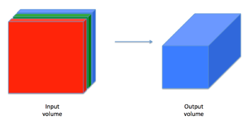
A convolution operation reduces an image (or generally: a previous layer) by applying a filter (a.k.a. kernel). This filter is a matrix that is being moved step by step over the image. In each step, all the elements of the image matrix that are being covered by the filter are multiplied with the corresnponding elements in the filter matrix. The products are then added up and the filter is moved into the next position. This process is repeated until all the pixels have been captured. A convolution operation is usually denoted by an asterisk *.

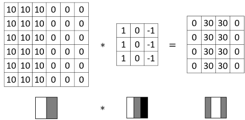
As you can see from above animation, the convolution operation results in a smaller matrix when no padding is used (we’ll talk about padding later). The parameters in the filter determine what feature is detected. For example consider the following picture (big matrix) and the filter (small matrix). High values in the image matrix mean brighter colors, and low values darker colors. By multiplying with the filter weights and adding the products up we get high values in a single convolution step if the values are big in the left partof the covered area and small on the right side. This filter is therefore able to detect vertical edges where the pixels on the left are bright and the pixels on the left and dark pixels on the right.

This example illustrates how the kernel encompasses a specific features. In the above examples vertical edges could be detected regardless of whether the bright pixels are on the left or right by using absolute values. Similarly, horizontal edges or generally edges of arbitrary angle could be detected with a suitable filter. However, the kernels are not usually set by hand but rather learned by the network. They can detect far more than straight edges, especially in deeper layer when the detected features can get very complex. We will see this in a later example.

Padding

In the above example the convolution operation resulted in a new matrix which was smaller than the input matrix. This is also called valid convolution. Assuming the input image was a matrix of dimensions $(n \times n)$ and the filter a matrix of dimensions $(f \times f)$ then the size of the matrix after convolution could be calculated with the following formula:

CNNs usually contain several convolution layers. However though, if we apply additional convolutions, the resulting matrices would become smaller and smaller. Additionally, we would lose the information from the matrix entries at the edges. This behavior is often not desired and can be corrected by using padding. By using padding we add additional $p$ pixels (more generally: matrix entries) around the image matrix. The values of those matrix entries can either be set to zero (zero-padding) or calculated by some other logic (e.g. average of the neighboring pixels). The following picture shows an example for zero-padding.

If we use a frame of $p$ pixels width for padding, formula $\ref{valid_convolution}$ can be rewritten to the following formula to calculate the new matrix size.

We can choose $p$ so that the resulting matrix has the same size as the input matrix. This is called same convolution. The formula to calculate $p$ for same convolution is:

Stride

Beside the hyperparameter $p$ for padding there is another hyperparameter $s$ for the stride. This value defines the step size to use in each convolution operation, i.e. the number of entries to move the filter in each step (step size). In the above examples we have assumed a value of $s=1$. We can expand formula $\ref{padding_convolution}$ to include an arbitrary stride as follows:

Note that rounding down the values is needed to prevent the resulting image size to take on fractional values.

Convolution over volumes

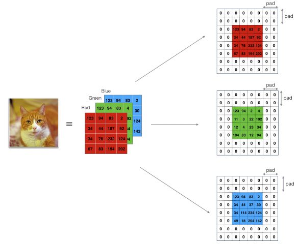
We have seen how convolution works for two-dimensional data. This would work for greyscale image, because they only contain one color channel. Usually images contain color in three channels (red, green and blue). Therefore the corresponding image matrices would also be three-dimensional (one two-dimensional matrix for each color channel).

Applying the convolution operation on three-dimensional matrices can be done by using a filter which is also three-dimensional. Generally speaking, in a convolution layer the filter dimensions should match the dimensions of the input matrices. This means if we apply a $5\times 5$-filter onto a $14 \times 14 \times 16$ matrix the filter’s dimension are by convention $( 5 \times 5 \times 16 )$. Such a filter can detect different features for the individual color channels. The convolution operation however works as seen above by moving the filter over the image, multiplying the elements and summing the products up. The resulting matrix is then again a two-dimensional matrix. However, we could apply more than one filter and stack the resulting matrices to get a multidimensional output matrix.

CONV-Layers

The first type of layer a CNN can have is the convolution layer, which applies the convolution operation as seen above. A convolution layer $l$ can therefore apply one or more filters to an input matrix. This gives us the following parameters for the layers:

• $f^{[l]}$: Kernel size
• $p^{[l]}$: Padding
• $s^{[l]}$: Stride
• $n_C^{[l]}$ Number of filters to apply
• $( n_H^{[l-1]} \times n_W^{[l-1]} \times n_C^{[l-1]} )$: Size of the input matrix
• $( f^{[l]} \times f^{[l]} \times n_C^{[l-l]} )$: Size of a matrix for a single kernel
• $( f^{[l]} \times f^{[l]} \times n_C^{[l-l]} \times n_C^{[l]} )$: Size of a matrix for all kernels
• $( n_H^{[l]} \times n_W^{[l]} \times n_C^{[l]} )$: Size of the output matrix for a single training sample
• $( m \times n_H^{[l]} \times n_W^{[l]} \times n_C^{[l]} )$: Size of the output matrix for a single training sample

The values of $n_H^{[l]}$ and $n_W^{[l]}$ can be calculated by the corresponding values from the previous layer:

Several convolutional layers can be combined to a Deep-CNN. The hyperparameters (size of the input or output matrix, number of filters, size of the filters, etc…) can be tuned with the following rules of thumb:

• the size of the input matrices (and therefore also the size of the output matrix should become smaller with increasing layer depth
• the number of channels should also decrease with each increasing layer depth

POOL-Layers

The second layer type in a CNN is the pooling layer. This layer is similar to the CONV layer in that a filter is slid over the input matrix. However, instead of multiplying the elements and summing up, the values for the output matrix are determined in a different way. There are two sub-types of this layer:

• Max-Pooling (POOL): The value in the output matrix corresponds to the maximum value in the covered area
• Average-Pooling (AVG): The value in the output matrix corresponds to the average value in the covered area

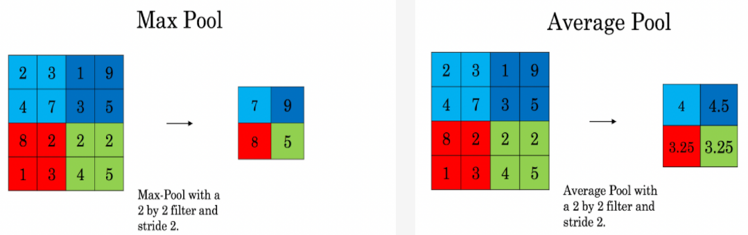
The pooling operation can be performed similar to the convolution operation by using different values for the stride. However, in contrast to the convolution operation, padding is usually not applied for pooling layers. Since there are no weights in the pooling filter there are no parameters to learn. Therefore, pooling layers usually reduce the input image in one or more dimensions. This is intentional because that way the CNN is forced to keep only the most important parameters.

FC-Layers

Usually when talking about the number of layers in a CNN only the layers with parameters (weights) are taken into account. Therefore, a pooling layer does not add to the network depth and can be considered belonging to the previous layer.

The last layer in a CNN is usually a layer of dimensions $(k \times 1)$ with all neurons connected to the previous layer (fully connected). This layer type is the same like we used in all NN so far. If neccessary, this vector can further be reduced to a $(t \times 1)$ vector ($t < k$) by multiplying it with a $(t \times k)$ matrix.

A CNN usually contains several CONV and POOL layers. A series of CONV layers is often followed by a single POOL layer. A typical CNN architecture is therefore the following:

CONV -> CONV -> ... -> POOL -> CONV -> CONV -> ... -> POOL -> FC -> FC -> ... -> FC -> Softmax

Advantages of convolutional layers

CONV layers have some advantages over FC layers:

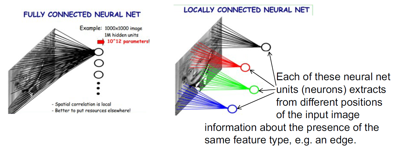
• Parameter sharing: A CONV layer needs to optimize less parameters than a FC layer because a lot of the parameters are shared. A feature detector that is useful in one part of the image is probably also useful in another part of the image.

• Sparsity of Connections: A value in the output matrix of a CONV layer only depends from a subset of the values in the input matrix. Therefore when performing backprop, a lot of parameters can be set to zero. This simplifies the calculation

Because a CNN has far less parameters to optimize than a CNN, a CNN also needs far less training data than a comparable Deep-NN without convolutional layers.

Case studies

Looking at existing network architectures are a good opportunity to see how others have designed their NN to solve a specific task. This can come in handy for problems where the results are transferreable (e.g. in Computer Vision).

Classic Networks

There are a few noteworthy CNN architectures that have had a big impact on Computer Vision or DL in general:

• LeNet-5
• AlexNet
• VGG-16

LeNet-5

LeNet-5 is a CNN with the following architecture:

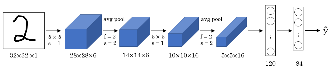
LeNet-5 was trained on the MNIST dataset, a collection of hand-written digits. This CNN is quite old and comparably small to current CNN (approximately 60k trainable parameters). It uses sigmoid or tanh as activation functions in the hidden layers. However, it does not use softmax as classifier in the last layer whereas today we probably would. We can further notice that it only uses valid convolutions (i.e. no padding) which results in the matrices becoming smaller and smaller.

AlexNet

AlexNet is a CNN with the following architecture:

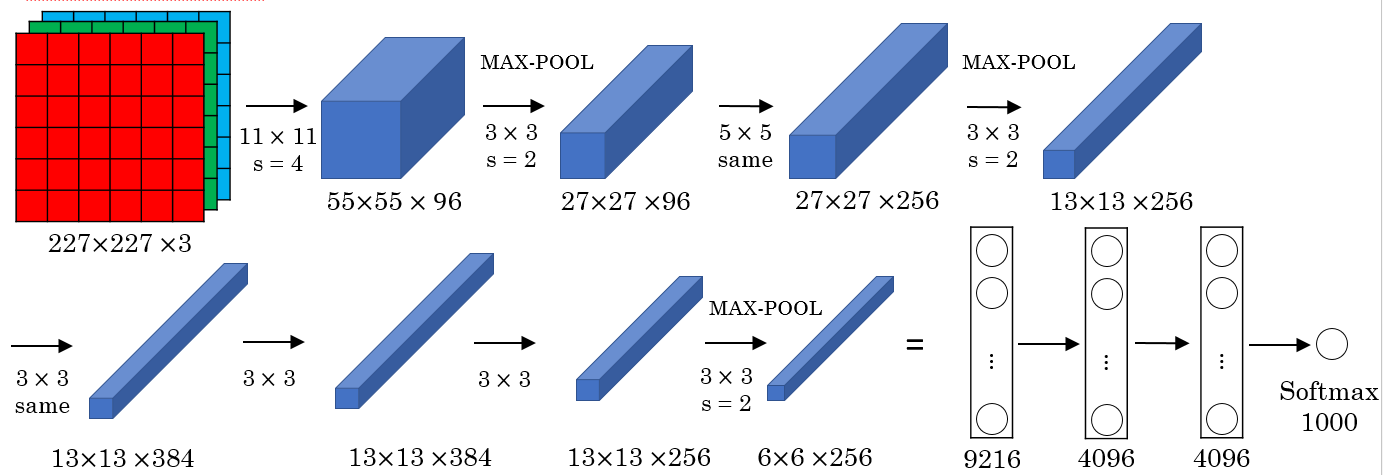
We can observe that AlexNet was trained on color images because it uses several channels in the input layer. Its architecture is similar to LeNet-5, but it is much bigger (approximately 60M trainable Parameters) and uses a so. It also uses ReLU as activation functions in the hidden layers and softmax as the classifier in the last layer. Its performance was far better than LeNet-5 which was an inspiration for scientists to use DL for computer vision.

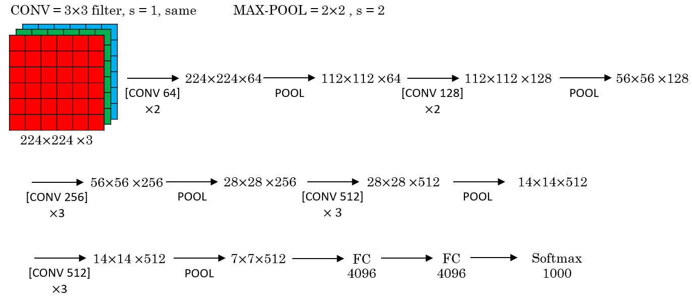
VGG-16

VGG-16 was a 16-Layer CNN with approximately 138M trainable parameters. The convolution layer all used SAME-convolution. Therefore the architecture is comparably simple (i.e. uniform and systematic). The following image shows a simplified representation of the 16 layers:

Residual Networks

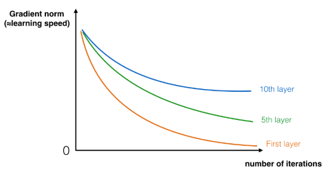
Recent Networks have become very deep. The CNN Microsoft used to win the ImageNet competition in 2015 was as deep as 152 layers! We have seen in part 2 that such a network usually suffers from vanishing (or in rare cases exploding) gradients and thus the gradient for the earlier layers decreases to zero very rapidly as training proceeds:

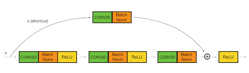
In order to train such very deep CNN that don’t suffer from exploding/vanishing gradient, we use special building blocks known as residual blocks. Those residual blocks consist of two conventional layer together with a shortcut (called skip-connection):

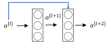
This residual block uses the activation of the previous layer $a^{[l]}$ for the calculation of its activation in the second layer. This calculation can be formally defined as:

If the weights inside the residual blocks become very small because of vanishing gradients, the activation of the previous layer dominates over the cell state during the calculation of the activation of the second layer. Therefore skip connections allow the forward propagation in a ResNet to learn some kind of identity function if the weights become too small. This makes learning the optimal parameters much simpler. If the input activation $a^{[l]}$ has the same dimensions as the output activation $a^{[l+2]}$ we call te residual block an identity block:

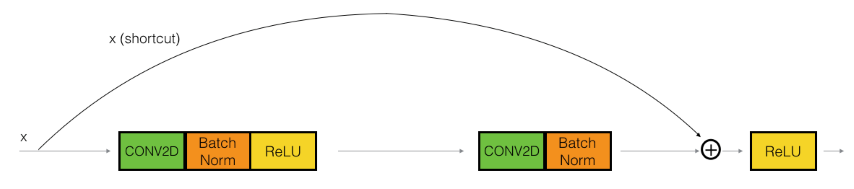
The upper path is the shortcut path, the lower the main path. However, the dimensions of the input and output activations do not neccessarily need to be the same. This is often the case when a skip-connection spans over more than 2 layers. In such cases we need the shortcut path to resize the input activation accordingly by applying a convolution operation to the input activation. Since the only purpose of this convolution is matching up the dimensions, the shortcut path does not use any non-linear activation function.

By stacking several of those residual blocks we get a ResNet that does not suffer from vanishing gradients anymore. In such a ResNet the danger of overfitting becomes much smaller. I.e. the error on the training data will gradually decrease whereas in contrast to conventional CNN it would increas again after a certain point.

1x1 convolutions

It can sometimes make sense to use a convolution layer with a kernel of dimensions $( 1 \times 1 \times n_C^{[l]})$ (wherer $n_C^{[l]}$ denotes the number of channels in the input layer). Such a layer can be used to reduce (or increase) the number of channels while preserving all the other dimensions. Generally, $n_C^{[l+1]}$ (the number of channels in the output layer) corresponds to the number of 1x1-filters applied to the input layer and can be set to any value. This is why 1x1 convolution layer are sometimes also referred to networks inside a network.

Inception modules

CONV- and POOL-operations can be applied simultaneiously in an inception module. The results of the individual operations can be stacked to appear as separate channels in the next layer.

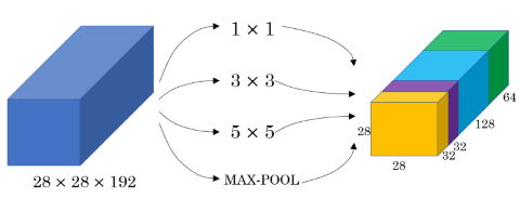
The values for $n_H$ and $n_W$ in the next layer are the same, but there are more channels. To achieve this, the POOL-layers must apply padding (which is usually only done for CONV-layers).

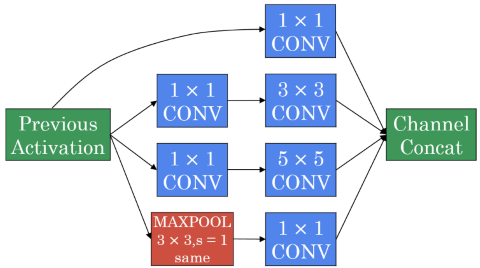
An inception module can also apply multiple CONV- and/or POOL-operations in a row to compute a batch of channels:

Computational cost

CNN however (especially CNN using inception modules) often require extremely high computational cost, because each element of the input layer needs to be multiplied with each element of a filter. Consider the following example of a convolution layer:

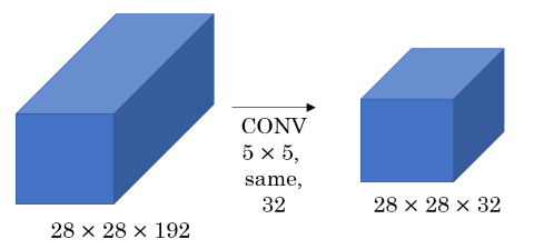
If we apply 32 convolution filters of dimensions $(5 \times 5 \times 192)$ each to an input layer of dimensions $(28 \times 28 \times 192)$ the number of multiplication operations is $(28 \cdot 2 \cdot 32) \cdot (5 \cdot 5 \cdot 32) \approx 120M$. To reduce this computational cost 1x1 convolutions are applied to reduce the input layer to a lower-dimensional intermediate matrix and apply the convolution to this intermediate matrix:

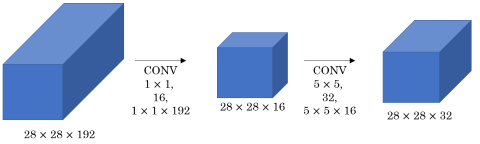
By using the intermediate matrix the number of operations for the first step is reduced to $(28 \cdot 28 \cdot 16) \cdot 192 \approx 2.4M$ and for the second step to $(28 \cdot 28 \cdot 32) \cdot (5 \cdot 5 \cdot 18) \approx 10M$ (total: $\approx 12.4M$ operations).

Surprisingly the predictive performance of the CNN does not suffer significantly by this reduction of computational cost. Multiple inception modules can be combined to form an inception network this way without the danger of exponentially increasing computational cost.

Practical advices for using ConvNets

It is sometimes useful to start out from the results of other researchers. Often however it is difficult to re-build a CNN from a paper from scratch. Luckily, the authors provide the pre-trained models and/or labelled data sets to train on for download. You can (and should) use those models for transfer learning. Additionally, if you only have little own training data to train on, you can use data augmentation to synthethizsize additional training data.

State of Computer Vision

Because for a lot of tasks in CV there is only very little labelled training data available, careful hand-engineering (of the CNN architecture, the features or other components) is very important to still get a reasonable data. This is different from other tasks where you can rely on a lot of training data to improve performance and spending a lot of time on hand-engineering might not be the way to go. The absence of abundant training data for very complex tasks might be the reason that some very complex network architectures have evolved especially in the area of computer vision. After training, the performance of a trained CNN can be verified on a benchmark dataset. A lot of competitions on Kaggle or other platforms are about beating an existing benchmark. Winning in such compoetitions might get you a lot of attention. There are some useful techniques to help beating the crowd in such competitions (although those are usually not applied in production because they are usually too expensive):

• Ensembling: Sometimes a good result on a benchmark dataset does not mean the CNN will apply well on unknown data. A (rarely used) possibility in such cases would be to train several (e.g. 3-15) CNN independently from another and then use the mean value of their outputs (not their weights!) to calculate the result.
• Multi-Crop at test time: A similar approach to ensembling is applying multi-cropping. Instead of training several networks and averaging their outputs you generate several variants of your image and average the results of a single network on each of the variants. In multi-cropping you crop your image to get the center piece, then move the cropping area to the corners to get the corner areas. This way you will get 5 crops out of your original image. You can mirror the image and apply the same process to get another five crops (10-crop-method). You can then classify each of the crops and calculate the average result of your network to get a prediction.

Detection algorithms

Besides classifying an image (i.e. labelling a picture with its content) it is often important to know where exactly on the picture the labelled object is. This is called object localization. Most of the time however we have more than one object on a single picture and not only want to know what objects there are but also where they are located. This is called object detection. Object detection is especially important in problem areas like autonomous driving where we usually label multiple objects (pedestrians, other cars, signs, red lights, etc.) inside an image and also want to know where they are.

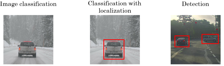
Object localization (OL)

To localize an object on an image we can use a bounding box with the following parameters:

• $b_x, b_y \in [0, 1]$: coordinates of the center of the bounding box (with the zero point being at the top left corner of the image)
• $b_H, b_W \in [0, 1]$: height and width of the bounding box (as ratios of the image size, i.e. a value of $b_W = 0.3$ means the box’ with is 30% of the image width)
• $p_c$: binary value whether the object is inside the picture or not

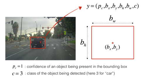
So far we used a one-hot representation to encode each object. The parameters of the bounding box can now be added to this encoding to get the vector representation of a single object:

Because the components $y_2 .. y_n$ of this vector are only relevant if the first component $y_1 = p_c = 1$ we can redefine our cost function as follows:

Note: This formula is the definition of the mean squared error loss function but also applies to other loss functions.

Landmark detection

Knowing an objects position on an image may be enough for applications like autonomous driving. However, for other problems this might not be enough. In face recognition for example it is not only important to know where the eyes, the nose, the mouth etc… are located, but also specific points of those body parts (e.g. the corners of the eyes). Such points are called landmarks and finding them is called landmark detection accordingly. It is important to notice that when working with landmarks detection the labelled landmarks have to be consistent over the training instances (e.g. landmark 1 for the left corner of the left eye, landmark 2 for the right corner of the left eye, and so on)

Object detection

In order to not only localize known objects but also find objects inside images one can work with sliding windows. A sliding window is successively moved over an image to analyze a part of the image in each step. While doing this the step size needs to be small enough so that an object is not skipped. The window size can be increased gradually to detect objects that would otherwise be too big to fit into the analyzed area.

This method of object recognition however is computationally very expensive and not feasible. A better implementation of a sliding window is its convolutional implementation. This involves turing fully connected layers into convolutional layers. To do this, consider the following example of a ConvNet with two FC layers:

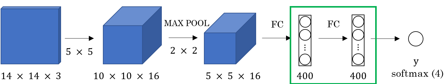
We can replace each of these FC layers with equivalent CONV layers by applying a filter that has the same dimensions as the input matrices. By using several of these filters (in this example: 400) we can create a CONV layer that is equivalent to the FC layer and has the same dimensionality in the third dimension

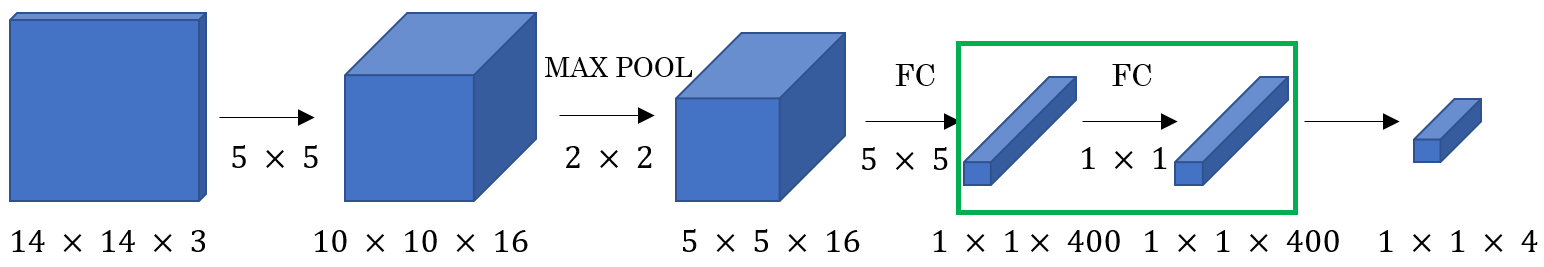
This method of replacing FC layers with equivalent CONV layers can be used to implement the sliding windows method by using convolution. Consider the following example of a ConvNet with an input image of size $14 \times 14 \times 3$ (note that the third dimension has been left out in the drawing for simplicity). This image is now convoluted by applying a $5 \times 5$ filter, some max-pooling and further convolution layers.

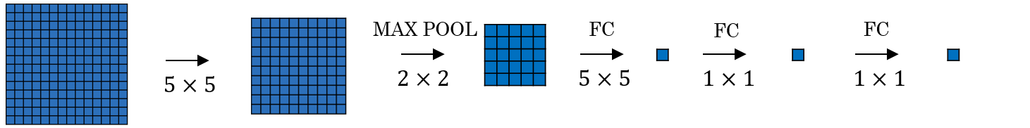
We can implement the sliding window method now by adding a border of two pixels to the left. This results in an input image of dimensions $16 \times 16 \times 3$. We can now apply the same $5 \times 5$ convolution and all the pooling and other pooling layers like before. However, because of the changed dimensions of the input image, the dimensions of the intermediate matrices are also different.

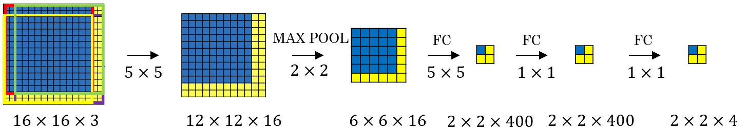
It turns out however that the upper left corner of the resulting matrix (blue square) is the result of the upper left area of the input image (blue area). The other square in the output matrix correspond to the other areas in the input image accordingly. This mapping applies to the intermediate matrices too. The advantage calculating the result convolutionally is that the forward propagations of all areas are combined into one form sharing a lot of the computation in the regions of the image that are common. In contrast, with the sliding window method as described above forward propagation would have been done several times independently (once for each position of the sliding window). A convolutional implementation of sliding windows has therefore considerable lower computational cost compared to a sequential implementation because all the positions of a sliding window are computed in a single forward pass.

YOLO

One disadvantage of the sliding windows method (even with a convolutional implementation) is that the window may not come to lie over an object nicely. That is there are only positions of the sliding window where parts of the object are outside the border of the window. Therefore the ConvNet cannot (or only badly) detect the object. One approach to solve this is the YOLO algorithm (You Only Look Once). This algorithm divides the image into multiple cells of equal size.

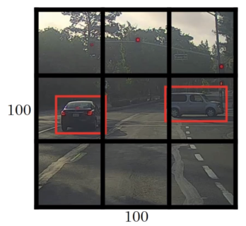
The basic idea is to then apply the sliding window process as described above to each of the cells. For this there must be labels for each grid cell encoded as label vectors as described in $\ref{label_vector}$. Whether an object belongs to a specific image segment or not is determined by the coordinates of the center of the bounding box. That way an object can only ever belong to exactly one segment.

In contrast to previously seen CNN the output for YOLO-networks is a volume, not a two-dimensional matrix. If we have for example 3 classes, the label vector would consist of 8 elements ($p_c, b_x, b_y, b_H, b_W, c_1, c_2, c_3$). If we divide the image into 9 segments as in the picture above we can detect one object per segment resulting in a label matrix (and therefore also the output matrix $Y$ of the CNN) of dimensions $( 3 \times 3 \times 8 )$. The following picture shows an example of a CNN that uses YOLO to divide an image into $19 \times 19$ segments and distinguishes between 80 classes and shows how it encodes an image:

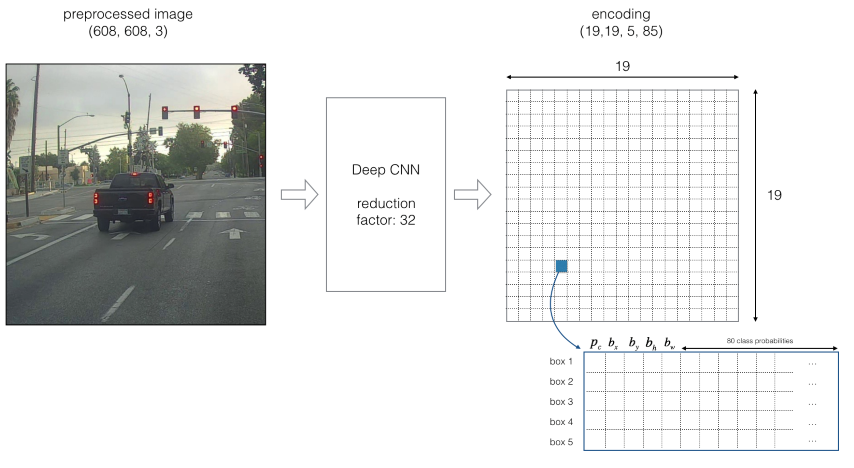
Note that the coordinates $b_x, b_y$ are relative to the grid cell, not the image. Therefore their values need to lie between 0 and 1. Likewise, the size of the bounding box (specified by $b_H$ and $b_W$) is relative to the size of the grid cell, but since the bounding box may overlap several grid cells those values can become greater than 1 (whereas in a different algorithm without segmentation the size of the bounding box cannot be greater than than the image).

The YOLO algorithm is a convolutional implementation of the sliding window method which makes it performant by sharing a lot of the computation. In fact, the YOLO algorithm is so performant that it can be used for real-time object detection.

Improvements to YOLO

There are a few ways to improve the performance of the YOLO algorithm.

• Intersection over union
• Non-max suppression
• anchor boxes

Intersection over union

An improvement of the YOLO algorithm can be achieved by calculating how much a predicted bounding box overlaps with the actual bounding box.

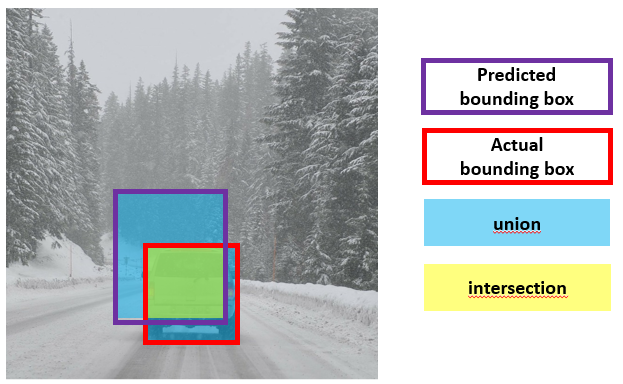
This value is called Intersection over Union (IoU) and can be more formally defined as:

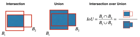
The IoU can be used to evaluate the accuracy of the localization. When $IoU > 0.5$ (or any reasonable value) the localization could be marked as correct.

Non-max supppression

YOLO can further be improved by using non-max suppression (NMS). NMS prevents YOLO from detecting the same object multiple times, e.g. if the YOLO algorithm calculates several bounding boxes for the same object with their center coordinates assigned to different cells. It does so by assigning the first component $p_c$ of a label vector (see $\ref{label_vector}$) a value between 0 and 1 (whereas before this value was binary, i.e. either 0 or 1). The value of $p_c$ corresponds to the confidence of the algorithm that the bounding box contains the respective object. NMS then searches for overlapping boxes and removes all but the one with the highest value of $p_c$. The following image illustrates this (the blue boxes are the ones that are removed, the green boxes are the ones that are retained):

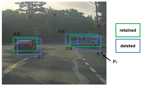
The algorithm for NMS is as follows:

1. Delete all bounding with $p_c$ below a threshold value (e.g. 0.6)
2. While there are bounding boxes:
   • Take the bounding box with the largest $p_c$. Output this as a prediction
   • Find all bounding boxes overlapping this bounding box ($IoU > 0.5$) and remove them

Anchor boxes

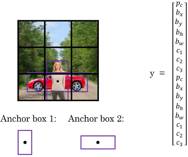
To enable the YOLO algorithm to detect more than one object per cell you can use anchor boxes. An anchor box corresponds to a bounding box for a certain object that overlaps the bounding box of another object. An object is assigned to the anchor box with the highes IoU value (whereas previously the object was assigned to the grid cell that contained the object’s midpoint). To predict more than one object per cell, the label-vectors need to be stacked on top of each other in the output. The following picture illustrates this for two anchor boxes (i.e. a YOLO-NN that can detect two objects per cell).

Putting it all together

Assume we train a ConvNet using YOLO by dividing the images with a $3 \times 3$ grid whereas the ConvNet should be able to detect 2 objects per grid cell and we have 3 possible classes of objects. The dimensions of the output matrix of such a ConvNet would therefore be $3 \times 3 \times (2 \cdot 8) = 3 \times 3 \times 16$.

Generally speaking the dimensions of the output $y$ of a ConvNet using YOLO with a $k \times l$ grid, $n_c$ classes and $m$ anchor boxes can be calculated as follows:

The term $(5 + n_c)$ stems from the five components needed to indicate the confidence and the coordinates/size of a bounding box ($p_c, b_x, b_y, b_H, b_W$) together with the $n_c$ components needed to form a one-hot vector of a class.

A CNN that uses YOLO can therefore do the following:

1. divide the picture into a grid of equally sized segments by using the YOLO-algorithm
2. detect and locate several objects in an image by applying a convolutional implementation of a sliding window
3. calculate the bounding boxes by training on the labelled data
4. use anchor-boxes to detect multiple different objects within the same grid cell
5. apply non-max suppression to keep only one bounding box per object
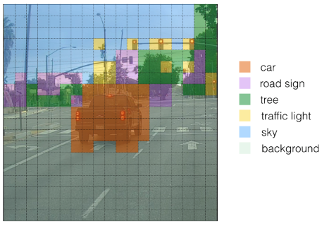
6. output a matrix of dimensions $dim(y)$ which represents the encoding of the information

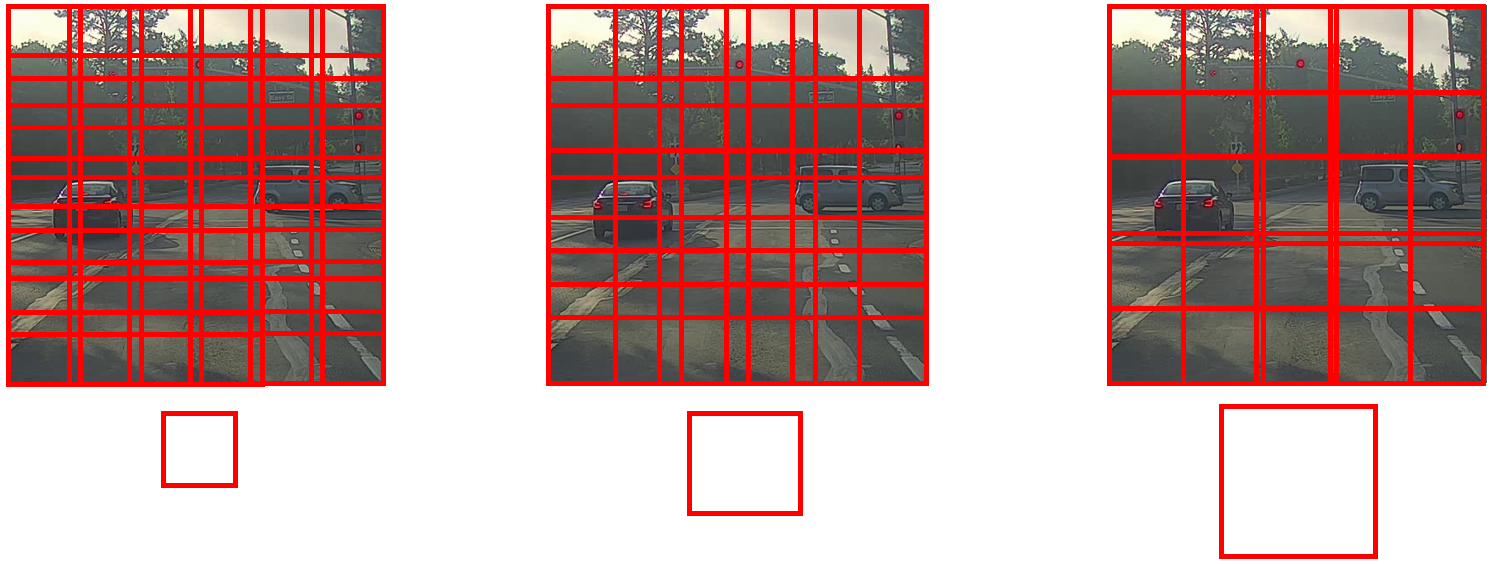
If we visualize the output matrix from the last step it might look something like this:

Face Recognition

One possible appliance of a CNN or Computer Vision in general is the face recognition. In face recognition we want to identify a person from a database of $K$ persons, i.e. we want a single input image to map to the ID of one of the $K$ persons in the database (or no output if the person was not recognized). This is different from face verification where we compare the input image only to a single persona and verify whether the input image is that of the claimed person.

One-shot learning

Up to this point we have only seen CNN that needed a lot of pictures to be trained. However, because we usually don’t have a lot of pictures of the same person, the problem with face recognition is that a CNN needs to be trained that is able to identify a person based on just a single picture. This process is called one-shot learning. Conventional CNN are not suitable for this kind of task, not only because they require a huge amount of training data, but also because the whole network would need to be re-trained if we want to identify a new person.

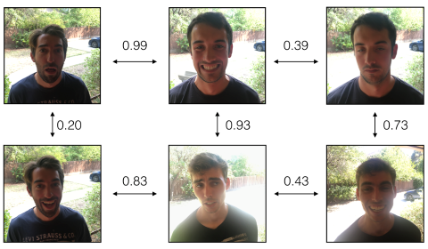
Instead when performing face recognition we apply a similarity function $d(x^{(i)} , x^{(j)})$ that is able to calculate the (dis)similarity between two images of persons $x^{(i)}$ and $x^{(j)}$ as a value $\tau$ (degree of difference). $\tau$ is small for persons who look alike and large for different persons:

Siamese networks

One way to implement this similarity function is a siamese network. Such a network encodes an input image as a vector of arbitrary dimensions (e.g. 128 components). The network can be understood as a function $f(x)$ that encodes an image $x$ whereas similar pictures lead to similar encodings.

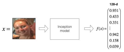
The similarity function can then be implemented as the vector norm of two image vectors:

Triplet loss

A siamese network should calculate similar image vectors for similar images and different vectors for different images. In other words: the distance between image vectors should be small for similar images and big for dissimilar images. We need to train the siamese network to exhibit this property. To do this we can use the triplet loss function (TLF). When using the TLF we define the image of one specific Person as anchor image $A$ and compare it with another image of the same person (positive image $P$) and an image of a different person (negative image $N$). Because of the initially formulated condition the following equation needs to hold true:

We can rearrange this equation and get:

However, there a catch with this equation: We could achieve it to be true by simply “calculating” the zero vector for each image! To prevent this, we add a parameter $\alpha$ and get:

By rearranging it back to the original form we get:

The parameter $\alpha$ is also called margin. The effect of this margin is that the value of $\tau$ for pictures of the same person differs a lot from pictures of different persons (i.e. $d(A,P)$ is separated from $d(A,N)$ by a big margin).

Considering all the points mentioned above we can define the TLF as follows:

Maximizing the two values prevents the network from calculating negative losses. The total cost can be calculated as usuall by summing the losses over all triplets:

Implications of TLF

The definition of the TLF function implies that in order to train a siamese network that exhibits the required properties we need at least two different images of the same person. To ensure a strong discrimination we should also consider triplets $(A,P,N)$ where $N$ is the image of a person who looks similar to $A$. That way we force the network to also learn to differentiate “hard” cases.

An alternative approach for facce recognition is to treat it as a binary classification problem. This could be used for an acces control system based on face recognition. We could store precomputed image vectors in a database and would only have to calculate/compare a person’s image vector. We can do this by training a CNN which calculates a value close to 1 for pictures of the same person and a value close to 0 for pictures of different persons. The calculation of this value could be as follows:

We could alternatively use the Chi-Squared-Similarity

Neural Style Transfer

Another interesting task in the field of Computer Vision is Neural Style Transfer (NST). NST takes a style image $S$ (e.g. a painting) and applies its style to a content image $C$ to produce a new image $G$. Because a new image is generated, a model that persforms NST is called a generative model.

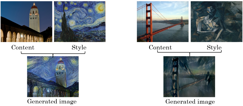
We can train such a model by training a NN that uses two cost functions:

• $J_{CONTENT}(C,G)$: Cost regarding the content of the original content image $C$ and the generated image $G$ (content cost function)
• $J_{STYLE}(S,G)$: Cost regarding the style of the original style image $S$ and the generated image $G$ (style cost function)

Both cost function can be combined to a single cost function:

This cost function can be minimized the same way as in regular NN. To do this, the image $G$ is initialized with random noise and then optimized by applying gradient descent to minimize the costs.

Content Cost

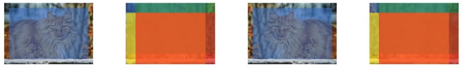
To understand how the content cost function works we can visualize what a deep NN is learning by inspecting the activations of neurons in different layers. By visualizing the image patches that maximally activate a neuron we can get a sense for what the neurons are learning. It turns out that the NN usually learns abstract things like “vertical edges”, “bright/dark” etc. in higher layers and more complex things like “water”, “dogs” etc. in deeper layers:

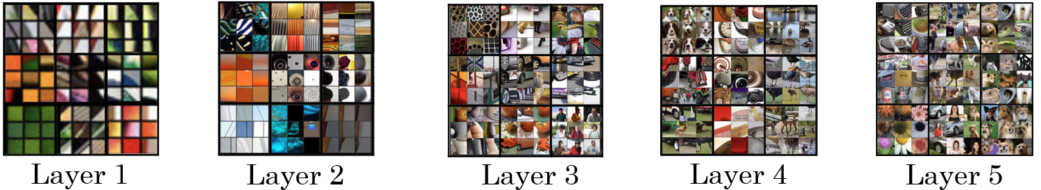
We can calculate the content cost at any layer in the network and thus control how big its influence is on the generated image. Let’s for example consider an image of a dog as the content image $C$. If we calculate the content cost in a higher layer we force the network to generate an image which looks similar to $C$. If we calculate the content cost in deeper layers we allow the network to generate an almost arbitrary image as long as there is a dog in the image. Usually some hidden layer in the middle is chosen to achieve a good balance between content and style.

Let $a^{[l](C)}$ and $a^{[l](G)}$ be the activations of layer $l$ for the content image $C$ or the style image $S$ respectively. The CCF can now be defined as the element-wise square difference:

Style Cost

To calculate the similarity between the styles of two images we can define style as the correlation between the activation across channels in a layer $l$. This correlation can be understood as follows:

• High correlation: An image patch which has a high value in both channel A and channel B contains a style property in both channels
• Low correlation: An image patch which ahs a high value in channel A and a small value in channel B (or vice versa) contains a style properties of channel A, but not the properties of channel B.

Let’s visualize this with an example. Consider the two high-level style properties “contains vertical lines” and “has an orange tint” which are reflected in different channels. If the two properties are highly correlated it means the original style image $G$ often contains vertical lines in conjunction with an orange tint. We can therefore measure the similarity in style of the generated image $G$ by checking if the correlation between these properties (channels) is high too.

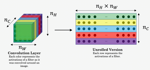
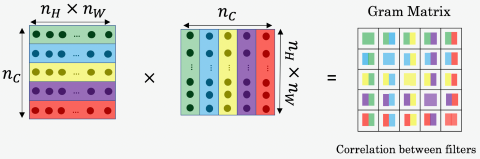
This can be expressed more formal as follows: Let $a^{[l]}_{i,j,k}$ be the activation of neuron $i$ in layer $l$ for the pixel at position $j,k$ in the style image $S$. We can represent the correlation between the $n_C$ channels in this layer as a style matrix G (a.k.a. Gram-Matrix) which has the dimensions $(n_c \times n_c)$. This is easiest if the image matrix is unrolled into a 2-dimensional matrix:

The elements of this matrix can thenbe calculated as follows:

This style matrix can be computed separately for both the style image $S$ and the generated image $G$. The SCF can then be defined as:

The SCF can be applied on different layers (low-level and high-level layers) whereas the results can be weighted by appliying a parameter $\lambda^{[l]}$ and summed up to get the overall style cost across all layers: